


Most data scientists/analysts using Python are familiar with the Pandas DataFrame library. And if you're in the data science field, you've probably invested quite a significant amount of time learning how to use the library to manipulate your data. One of the main complaints about Pandas is its slow speed and inefficiencies when dealing with large datasets. Fortunately, there's a new DataFrame library that attempts to address this main complaint about Pandas called Polars.
Polars is a DataFrame library completely written in Rust. In this article, I'll walk you through the basics of Polars and how it can be used in place of Pandas.
What Is Polars?
The best way to understand Polars is that it's a better DataFrame library than Pandas. Here are some advantages of Polars over Pandas:
- Polars does not use an index for the DataFrame. Eliminating the index makes it much easier to manipulate the DataFrame. The index is mostly redundant in Pandas' DataFrame anyway.
- Polars represents data internally using Apache Arrow arrays while Pandas stores data internally using NumPy arrays. Apache Arrow arrays is much more efficient in areas like load time, memory usage, and computation.
- Polars supports more parallel operations than Pandas. As Polars is written in Rust, it can run many operations in parallel.
- Polars supports lazy evaluation. Polars examines your queries, optimizes them, and looks for ways to accelerate the query or reduce memory usage. Pandas, on the other hand, support only eager evaluation, which immediately evaluates an expression as soon as it encounters one.
Installing Polars
To install Polars, use the pip command:
$ pip install polars
Or, use the conda command:
$ conda install polars
For this article, I'm going to assume that you have Anaconda installed and that you are familiar with Jupyter Notebook.
If you are new to Jupyter Notebook, check out this introduction to Jupyter Notebook at https://jupyter.org/try-jupyter/retro/notebooks/?path=notebooks/Intro.ipynb.
Creating a Polars DataFrame
The best way to learn a new library is to get your hands dirty. Let's get started by importing the polars module and creating a Polars DataFrame:
import polars as pl
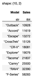
df = pl.DataFrame(
{
'Company': ['Ford','Toyota','Toyota','Honda','Toyota',
'Ford','Honda','Subaru','Ford','Subaru'],
'Model': ['F-Series','RAV4','Camry','CR-V','Tacoma',
'Explorer','Accord','CrossTrek','Escape','Outback'],
'Sales': [58283,32390,25500,18081,21837,19076,11619,15126,
13272,10928]
}
)
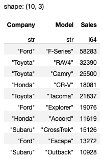
df
Like Pandas, Polars automatically pretty-prints (displayed using a CSS stylesheet) the DataFrame when it's displayed in Jupyter Notebook (see Figure 1).
Polars expects the column header names to be of string type. Consider the following example:
df2 = pl.DataFrame(
    {
        0 : [1,2,3],
        1 : [80,170,130],
    }
)
The above code snippet won't work as the keys in the dictionary are of type integer (0 and 1). To make it work, you need to make sure the keys are of string type (“0” and “1”):
df2 = pl.DataFrame(
    {
        "0" : [1,2,3],
        "1" : [80,170,130],
    }
)
Besides displaying the header name for each column, Polars also displays the data type of each column. If you want to explicitly display the data type of each column, use the dtypes properties:
df.dtypes
For the df example, you see the following output:
[polars.datatypes.Utf8,
 polars.datatypes.Utf8,
 polars.datatypes.Int64]
To get the column names, use the columns property:
df.columns
# ['Company', 'Model', 'Sales']
To get the content of the DataFrame as a list of tuples, use the rows() method:
df.rows()
For the above df example, you see the following output:
[('Ford', 'F-Series', 58283),
 ('Toyota', 'RAV4', 32390),
 ('Toyota', 'Camry', 25500),
 ('Honda', 'CR-V', 18081),
 ('Toyota', 'Tacoma', 21837),
 ('Ford', 'Explorer', 19076),
 ('Honda', 'Accord', 11619),
 ('Subaru', 'CrossTrek', 15126),
 ('Ford', 'Escape', 13272),
 ('Subaru', 'Outback', 10928)]
Polars doesn't have the concept of index, unlike Pandas. The design philosophy of Polars explicitly states that index isn't useful in DataFrames.
Selecting Column(s)
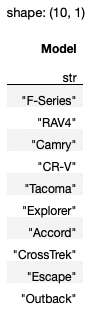
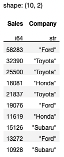
Selecting column(s) in Polars is straightforward - simply specify the column name using the select() method:
df.select(
    'Model'
)
The above statement returns a Polars DataFrame containing the Model column (see Figure 2).
Polars also supports the square bracket indexing method, the method that most Pandas developers are familiar with. However, the documentation for Polars specifically mentions that the square bracket indexing method is an anti-pattern for Polars. Although you can do the above using df[:,[0]], there's a possibility that the square bracket indexing method may be removed in a future version of Polars.
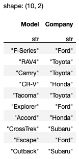
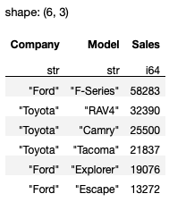
If you want multiple columns, supply the column names as a list:
df.select(
    ['Model', 'Company']
)
The output is as shown in Figure 3.
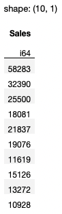
If you want to retrieve all the integer (specifically Int64) columns in the DataFrame, you can use an expression within the select() method:
df.select(
    pl.col(pl.Int64)  # all Int64 columns
)
The statement pl.col(pl.Int64) is known as an expression in Polars. This expression is interpreted as “get me all the columns whose data type is Int64.” The above code snippet produces the output as shown in Figure 4.
Expressions are very powerful in Polars. For example, you can pipe together expressions, like this:
df.select(
    pl.col(['Model','Sales'])
    .sort_by('Sales'))
The result is a DataFrame that contains two columns, sorted based on the values in the Sales column (see Figure 5).
If you want multiple columns, you can enclose your expression in a list:
df.select(
    [pl.col(pl.Int64), 'Company']
)
Figure 6 shows the result of this query.
If you want to get all the string-type columns, use the pl.Utf8 property:
df.select(
    [pl.col(pl.Utf8)]
)
Selecting Row(s)
To select a single row in a DataFrame, pass in the row number using the row() method:
df.row(0) # get the first row
The result is a tuple:
('Ford', 'F-Series', 58283)
If you need to get multiple rows based on row numbers, you need to use the square bracket indexing method, although it is not the recommended way to do it in Polars. Here are some examples:
df[:2]          # first 2 rows
df[[1,3]]       # second and fourth row
To select multiple rows, Polars recommends using the filter() function. For example, if you want to retrieve all Toyota's cars from the DataFrame, you can use the following expression:
df.filter(
    pl.col('Company') == 'Toyota'
)
You can also specify multiple conditions using logical operators:
df.filter(
    (pl.col('Company') == 'Toyota') | (pl.col('Company') == 'Ford')
)
The result now contains all cars from Toyota and Ford (see Figure 7).
You can use the following logical operators in Polars: | (or), & (and), and ~ (not).
Selecting Rows and Columns
Very often, you need to select rows and columns at the same time. You can do so by chaining the filter() and select() methods, like this:
df.filter(
    pl.col('Company') == 'Toyota'
).select('Model')
The above statement selects all the rows containing Toyota and then only shows the Model column. If you also want to display the Sales column, pass in a list to the select() method:
df.filter(
    pl.col('Company') == 'Toyota'
).select(['Model','Sales'])
Quick Tip: Use
select()to choose columns and usefilter()to choose rows from a Polars DataFrame.
Understanding Lazy Evaluation
The key advantage of Polars over Pandas is its support for lazy evaluation. Lazy evaluation allows the library to analyze and optimize all of the queries before it starts executing any of the queries. By doing so, the library can save a lot of time by reducing the amount of work processing redundant operations.
Implicit Lazy Evaluation
To understand the effectiveness of lazy evaluation, it's useful to compare to how things are done in Pandas. For this exercise, I'm going to use the flights.csv file located at https://www.kaggle.com/datasets/usdot/flight-delays. This dataset contains the flight delays and cancellation details for flights in the U.S. in 2015. It was collected and published by the Department of Transportation's Bureau of Transportation Statistics.
I'll use Pandas to load the flights.csv file, which contains 5.8 million rows and 31 columns. Usually, if you load this on a computer with limited memory, Pandas takes a long time to load it into a DataFrame (if it loads at all). This code does the following:
- Loads the
flights.csvfile into a Pandas DataFrame - Filters the DataFrame to look for those flights in December and whose origin airport is SEA and destination airport is DFW
- Measures the amount of time needed to load the
CSVfile into a DataFrame and does the filtering
import pandas as pd
import time

start = time.time()
df = pd.read_csv('flights.csv')
df = df[(df['MONTH'] == 12) &
        (df['ORIGIN_AIRPORT'] == 'SEA') &
        (df['DESTINATION_AIRPORT'] == 'DFW')]

end = time.time()
print(end - start)
df
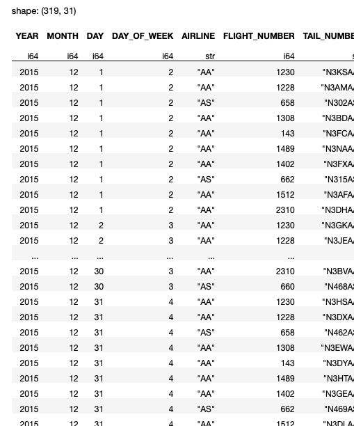
On my Mac Studio with 32GB RAM, the above code snippet took about 6.1 seconds to load and displays the result as shown in Figure 8.
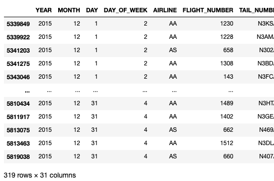
The main issue with Pandas is that you had to load all the rows of the dataset into the DataFrame before you could do any filtering to remove all the unwanted rows. Although you can load the first or last n rows of a dataset into a Pandas DataFrame, to load specific rows (based on certain conditions) into a DataFrame requires you to load the entire dataset before you can perform the necessary filtering. This is the Achilles' heel of Pandas.
Let's now use Polars and see if the loading time can be reduced. The following code snippet does the following:
- Load the CSV file using the
read_csv()method of the Polars library. - Perform a filter using the
filter()method and specify the conditions for retaining the rows that you want.
import polars as pl
import time
start = time.time()
df = pl.read_csv('flights.csv').filter(
     (pl.col('MONTH') == 12) &
     (pl.col('ORIGIN_AIRPORT') == 'SEA') &
     (pl.col('DESTINATION_AIRPORT') == 'DFW'))
end = time.time()

print(end - start)
display(df)
On my computer, the above code snippet took about 0.6 seconds, a vast improvement over Pandas (see Figure 9).
It's important to know that the read_csv() method uses eager execution mode, which means that it will straight-away load the entire dataset into the DataFrame before it performs any filtering. In this aspect, this block of code that uses Polars is similar to that of that using Pandas. But you can already see that Polars is much faster than Pandas.
Notice here that the filter() method works on a Polars DataFrame object.
The next improvement is to replace the read_csv() method with one that uses lazy execution: scan_csv(). The scan_csv() method delays execution until the collect() method is called. It analyzes all the queries right up until the collect() method and tries to optimize the operation. The following code snippet shows how to use the scan_csv() method together with the collect() method:
import polars as pl
import time

start = time.time()
df = pl.scan_csv('flights.csv').filter(
        (pl.col('MONTH') == 12) &
        (pl.col('ORIGIN_AIRPORT') == 'SEA') &
        (pl.col('DESTINATION_AIRPORT') == 'DFW')).collect()
end = time.time()
print(end - start)
display(df)
The scan_csv() method is known as an implicit lazy method, because, by default, it uses lazy evaluation. It's important to remember that the scan_csv() method doesn't return a DataFrame object - instead it returns a LazyFrame object. And so, in this case, the filter() method actually works on a Polars LazyFrame object instead of a DataFrame object.
For the above code snippet, instead of loading all the rows into the DataFrame, Polars optimizes the query and loads only those rows satisfying the conditions in the filter() method. On my computer, the above code snippet took about 0.3 seconds, a further reduction in processing time compared to the previous code snippet.
Explicit Lazy Evaluation
Remember earlier on I mentioned that the read_csv() method uses eager execution mode? What if you want to use lazy execution mode on all its subsequent queries? Well, you can simply call the lazy() method on it and then end the entire expression using the collect() method, like this:
import polars as pl
import time

start = time.time()
df = pl.read_csv('flights.csv')
      .lazy()
      .filter(
        (pl.col('MONTH') == 12) &
        (pl.col('ORIGIN_AIRPORT') == 'SEA') &
        (pl.col('DESTINATION_AIRPORT') == 'DFW')).collect()
end = time.time()

print(end - start)
display(df)
By using the lazy() method, you're instructing Polars to hold on the execution for subsequent queries and instead optimize all the queries right up to the collect() method. The collect() method starts the execution and collects the result into a DataFrame. Essentially, this method instructs Polars to eagerly execute the query.
Understanding the LazyFrame object
Let's now break down a query and see how Polars works. First, let's use the scan_csv() method and see what it returns:
pl.scan_csv('titanic_train.csv')
The data source for this dataset is from https://www.kaggle.com/datasets/tedllh/titanic-train.
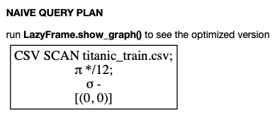
The above statement returns a LazyFrame object. In Jupyter Notebook, it shows the execution graph (see Figure 10).
Note that if you don't see the figure as shown, you need to install the pydot and graphviz packages as follows:
$ conda install pydot
$ conda install graphviz
The execution graph shows the sequence in which Polars executes your query. The LazyFrame object that's returned represents the query that you've formulated but not yet executed. To execute the query, you need to use the collect() method:
pl.scan_csv('titanic_train.csv').collect()
You can also enclose the query using a pair of parentheses and assign it to a variable. To execute the query, you simply call the collect() method of the query, like this:
q = (
     pl.scan_csv('titanic_train.csv')
)
q.collect()
The advantage of enclosing your queries in a pair of parentheses is that it allows you to chain multiple queries and put them in separate lines, thereby greatly enhancing readability. The above code snippet shows the output as shown in Figure 11.
For debugging purposes, sometimes it's useful to just return a few rows to examine the output, and so you can use the fetch() method to return the first n-rows:
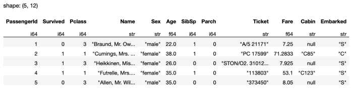
q.fetch(5)
The above statement returns the first five rows of the result (see Figure 12).
You can chain the various methods in a single query:
q = (
    pl.scan_csv('titanic_train.csv')
    .select(['Survived', 'Age'])
    .filter(
        pl.col('Age') > 18
    )
)
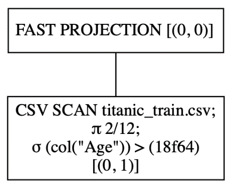
The show_graph() method displays the execution graph that you've seen earlier, with a parameter to indicate if you want to see the optimized graph:
q.show_graph(optimized=True)
The above statement shows the following execution graph. You can see that the filtering based on the Age column is done together during the loading of the CSV file (see Figure 13).
In contrast, let's see how the execution flow will look if the queries are executed in eager mode (i.e., non-optimized):
q.show_graph(optimized=False)
As you can see from the output in Figure 14, the CSV file is first loaded, followed by the selection of the two columns, and finally, the filtering is performed.

To execute the query, call the collect() method:
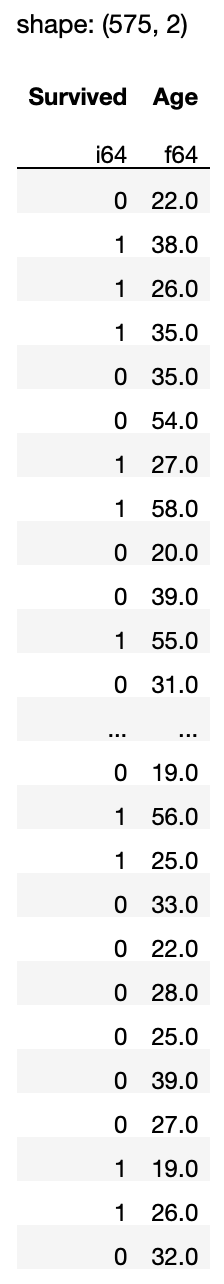
q.collect()
The output in Figure 15 shows all the passengers on the Titanic whose age is more than 18.
If you only want the first five rows, call the fetch() method:
q.fetch(5)
Data Cleansing
Now that you've learned the basics of Polars, let's focus on something that data scientists spend their most time doing: data cleansing. Data cleansing is the process of detecting and correcting corrupt values in your dataset. In real life, this seemingly simple process takes a lot of time as most of the data that you encounter is likely to contain missing values, incorrect values, or irrelevant values.
Loading the DataFrame
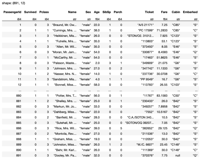
For this section, I'll continue to use the Titanic dataset. First, load the CSV into a Polars DataFrame:
import polars as pl
q = (
pl.scan_csv('titanic_train.csv')
)
df = q.collect()
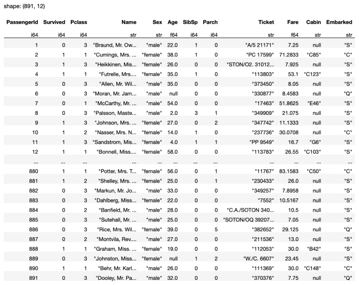
df
The DataFrame contains 891 rows with 12 columns. Notice the null values in the DataFrame shown in Figure 16.

All missing values in the CSV file will be loaded as null in the Polars DataFrame.
Looking for Null Values
To check for null values in a specific column, use the select() method to select the column and then call the is_null() method:
import polars as pl
q = (
    pl.scan_csv('titanic_train.csv')
    .select(pl.col('Cabin').is_null())
)

df = q.collect()
df
The is_null() method returns the result as a DataFrame of Boolean values.
Counting the Number of Null Values
It would be more useful to know how many rows in the column have null values, rather than seeing a DataFrame full of Boolean values. Hence, you can use the sum() method:
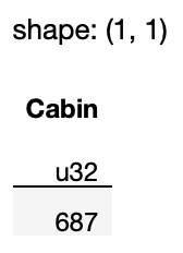
q = (
    pl.scan_csv('titanic_train.csv')
    .select(pl.col('Cabin').is_null().sum())
)
As you can see from the result in Figure 17, the Cabin column has 687 null values:
The difference between
sum()andcount()is that thesum()method only sums those values that aretrue, whereas thecount()method sums all values, includingfalse.
If you want to know if any of the values in the column contain null, use the any() method:
.select(
    pl.col('Cabin').is_null().any()
)
# returns True
Likewise, to see if all the values in the columns are null, use the all() method:
.select(
    pl.col('Cabin').is_null().all()
)
# returns False
Counting the Number of Null Values for Each Column in the DataFrame
Often, you want to have a quick glance at which columns in a DataFrame contain null values, instead of checking each column one by one. It would be useful to iterate through the columns and print the results. You can fetch all the columns in a DataFrame by calling the get_columns() method and then iterating through it:
q = (
    pl.scan_csv('titanic_train.csv')
)

for col in q.collect(): print(f'{col.name} - {col.is_null().sum()}')
The above code snippet prints out the following output:
PassengerId - 0
Survived - 0
Pclass - 0
Name - 0
Sex - 0
Age - 177
SibSp - 0
Parch - 0
Ticket - 0
Fare - 0
Cabin - 687
Embarked - 2
You can see that the following columns contain null values:
- Age
- Cabin
- Embarked
Replacing Null Values
Once you have determined which columns contain null values, the next logical step is to:
- Fill in the null values with some other values.
- Remove rows that contain null values.
Filling in the Entire Dataframe
You can fill the null values in the entire DataFrame using the fill_null() method:
q = (
    pl.scan_csv('titanic_train.csv')
    .fill_null(strategy='backward')
)
q.collect()
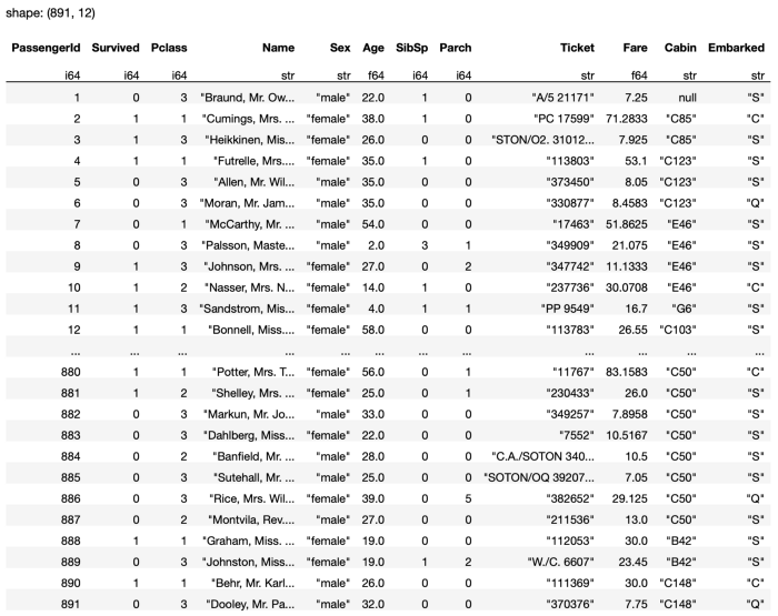
In the above statement, I used the backward-fill strategy, where all the null values are filled with the next non-null value (see Figure 18 for the output).
Notice that the last row contains a null value for the Cabin column. This is because it doesn't have a next row for it to reference a value to fill.
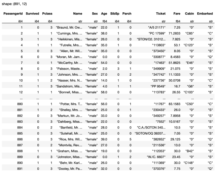
You can also use the forward-fill strategy, where all null values are filled with the previous non-null values:
q = (
    pl.scan_csv('titanic_train.csv')
    .fill_null(strategy='forward')
)
The output for the above statement is as shown in Figure 19.
Now you will realize that the Cabin value for the first row is null as it doesn't have a previous row to reference the value to fill.
You can also fill the null values with a fixed value, such as 0:
q = (
    pl.scan_csv('titanic_train.csv')
    .fill_null(0)
)
The output for the above statement is as shown in Figure 20.
Filling in a Specific Column
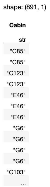
More often than not, you'd adopt different fill values for different columns, depending on the data type of the column. For example, you can fill the Cabin column using the backward-fill strategy:
q = (
    pl.scan_csv('titanic_train.csv')
    .select(pl.col('Cabin')
    .fill_null(strategy='backward'))
)
Notice that the above statement returns a DataFrame containing just the Cabin column (see Figure 21).
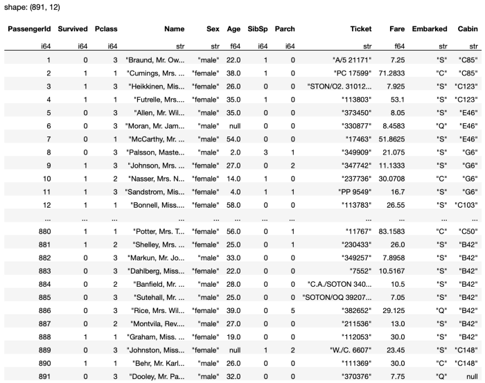
If you want to include the other columns in the DataFrame, add the following statement that includes the braces [ ]:
q = (
    pl.scan_csv('titanic_train.csv')
    .select(
        [
            pl.exclude('Cabin'),
            # select all columns except Cabin
            pl.col('Cabin').fill_null(strategy='backward')
        ]
    )
)
The entire DataFrame is now returned (see Figure 22).
You can also replace the null values in a specific column with a fixed value:
q = (
    pl.scan_csv('titanic_train.csv')
    .select(
        [
           pl.exclude('Age'),
           pl.col('Age').fill_null(value = 0)
        ]
    )
)
Or replace them with the mean of the column:
q = (
    pl.scan_csv('titanic_train.csv')
    .select(
        [
            pl.exclude('Age'),
            pl.col('Age').fill_null(value = pl.col('Age').mean())
        ]
    )
)
q.collect()
What if you want to replace a null value with the most frequently occurring value in the column? For example, for the Embarked column, you want to replace the null values with the port that most passengers embarked from. In this case, you can use the mode() method:
q = (
    pl.scan_csv('titanic_train.csv')
    .select(
        [
            pl.exclude('Embarked'),
            pl.col('Embarked').fill_null(
            value=pl.col('Embarked').mode())
        ]
    )
)
q.collect()
The mode() method returns the most frequently occurring value in a column.
Note that mode() doesn't work on floating-point columns.
Dropping Rows and Columns
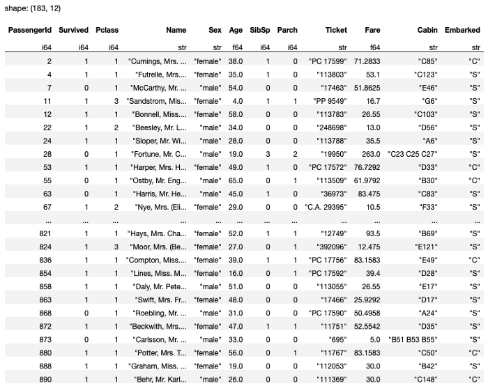
Sometimes it just makes sense to drop rows when there are null values in your DataFrame, especially when the number of rows with null values are small relative to the total number of rows you have. To drop all rows in the entire DataFrame with null values, use the drop_nulls() method:
q = (
    pl.scan_csv('titanic_train.csv').drop_nulls()
)
q.collect()
Note that after doing this, the result is left with 183 rows (see Figure 23).
In this dataset, it's not really a good idea to do this as the Cabin column has the most number of null values. Hence you should really drop the Cabin column instead, like this:
q = (
    pl.scan_csv('titanic_train.csv')
    .select(pl.exclude('Cabin'))
)
q.collect()
You can also use the drop() method to drop one or more columns:
# drop the Cabin column
q = (
    pl.scan_csv('titanic_train.csv').drop(['Cabin'])
)
q.collect()

# drop the Ticket and Fare columns
q = (
    pl.scan_csv('titanic_train.csv').drop(['Ticket', 'Fare'])
)
q.collect()
Notice that the drop() method doesn't modify the original DataFrame: It simply returns the DataFrame with the specified column(s) dropped. If you want to modify the original DataFrame, use the drop_in_place() method:
df = pl.read_csv('titanic_train.csv')
df.drop_in_place('Ticket')
Note that the drop_in_place() method can only drop a single column. It returns the dropped column as a Polars Series.
Note that you can only call
drop_in_place()on a Polars DataFrame, but not on a LazyFrame.
For the drop_null() method, you can also drop rows based on specific columns, using the subset parameter:
q = (
    pl.scan_csv('titanic_train.csv')
    .drop_nulls(subset=['Age','Embarked'])
)
q.collect()
In this case, only rows with null values in the Age and Embarked columns will be dropped.
You can also call the drop_nulls() method directly on specific columns:
q = (
    pl.scan_csv('titanic_train.csv')
    .select(pl.col(['Embarked']).drop_nulls())
)
q.collect()
In this case, the result will be a DataFrame containing the Embarked column with the null values removed.
Removing Duplicate Values
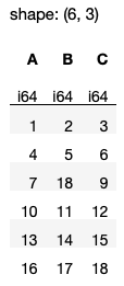
The final data cleansing technique that I'll discuss in this article is that of removing duplicates. For this example, I'll manually create a Polars DataFrame (see Figure 24 for the output):
import polars as pl

df = pl.DataFrame(
    {
         "A": [1,4,4,7,7,10,10,13,16],
         "B": [2,5,5,8,18,11,11,14,17],
         "C": [3,6,6,9,9,12,12,15,18]
    }
)
df
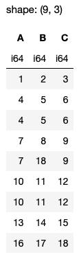
Observe that there are a few duplicated rows, e.g., 4, 5, 6 as well as 10, 11, 12. Additionally, there are rows where values for columns A and C are duplicates, e.g., 7, 9.
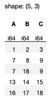
Using the unique() Method
First, let's remove the duplicates using the unique() method (see Figure 25 for output):
df.unique()
You can also use the distinct() method. However, it's since been deprecated in version 0.13.13 of Polars and it's not recommended to use it.
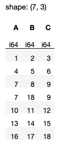
Observe from the output that if you don't supply any argument to the unique() method, all the duplicating rows will be removed and only one row will be kept.
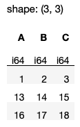
You can also remove duplicates based on specific columns using the subset parameter (see Figure 26 for the output):
df.unique(subset=['A','C'], keep='first')
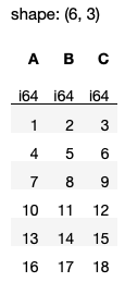
In the above result, observe that the row 7, 8, 9 is kept while the next row 7, 18, 9 is removed. This is because for these two rows, they have duplicate values for columns A and C. The keep='first' argument (default argument value) keeps the first duplicate row and removes the rest.
If you want to keep the last duplicate row, set keep to ‘last’ (see Figure 27 for output):
df.unique(subset=['A','C'], keep='last')
Observe that the row 7, 18, 9 will now be kept.
Removing All Duplicate Rows
What about removing all duplicate rows in Polars? Unlike in Pandas where you can set the keep parameter in the drop_duplicates() method to False to remove all duplicate rows:
# assuming df is a Pandas DataFrame
df.drop_duplicates(keep=False)
The keep parameter in the unique() method in Polars doesn't accept the False value. So if you want to remove duplicate values, you have to do things a little differently.
First, you can use the is_duplicated() method to get a Series result indicating which rows in the DataFrame are duplicates:
df.is_duplicated()
You will get a result, as follows:
shape: (9,)
Series: '' [bool]
[false
 True
 True
 False
 False
 True
 True
 False
 False
]
To fetch all those non-duplicate rows (essentially dropping all duplicate rows), you can use the square bracket indexing method:
df[~df.is_duplicated()]
But because square bracket indexing method is not recommended in Polars, you should use a more Polars-friendly method. You can do this using the filter() and pl.lit() methods:
df.filter(
    pl.lit(~df.is_duplicated())
)
All rows with duplicate values are now removed (see Figure 28).
Finally, if you want to remove all duplicates based on specific columns, you can simply use the pl.col() method and pass in the specific column names:
df.filter(    ~
.col(['A','C']).is_duplicated()
)
The above statement generates the output as shown in Figure 29.
Summary
In this article, I've given you a quick introduction to the Polars DataFrame library. The most exciting feature of Polars is its lazy evaluation mode, which optimizes your queries. This results in faster processing of large datasets, as well as less memory required. I hope the examples provided an easy way for you to get jumpstarted with this new and exciting library. Let the battle of the bears begin!
