Microsoft SQL Server 2012 Management and Administration, 2nd Edition, Chapter 2 - Administering Storage, I/O, and Partitioning in Microsoft SQL Server 2012

By Ross Mistry, Shirmattie Seenarine, Published Sep 18, 2012 by Sams. Copyright 2013, Dimensions: 5-3/8" x 8-1/4", ISBN-10: 0-672-33600-6, ISBN-13: 978-0-672-33600-3. Sample Chapter is provided courtesy of Sams Publishing. Click here to purchase book. http://www.informit.com/store/microsoft-sql-server-2012-management-and-administration-9780672336003

This chapter focuses on the use and most effective configuration of storage components within a Database Engine instance of SQL Server 2012.

Storage and I/O (input/output) within SQL Server 2012 requires special attention because it is perhaps the most likely subsystem to experience suboptimal performance when left to the default settings. As a consequence, the well-prepared DBA will want to spend a bit of extra time in planning, configuring, and tuning SQL Server’s storage and I/O settings.

This chapter introduces the fundamental concepts around SQL Server storage and I/O configuration and tuning. This overview includes hardware-related topics, such as hard disks, RAID, and SAN. Going beyond overview, this chapter will delve into the best practices and industry standards for SQL Server administrator activities, such as the number and placement of database and transaction log files, partitions, and tempdb configuration.

Most features related to SQL Server storage and I/O are configured and administered at the database level. That means that administrative tasks in SQL Server Management Studio will typically focus on database-level objects in the Object Explorer, as well as on database properties. Toward the end of this chapter, an important I/O performance-enhancing feature, data compression, is also discussed.

Even though the chapter introduces and explains all the administration and configuration principles of the SQL Server 2012 Storage Engine, you will occasionally be directed to other chapters for additional information. This is a result of the Storage Engine feature being so large and intricately connected to other features.

What’s New for DBAs When Administering Storage on SQL Server 2012

SQL Server 2012 enhances the functionality and scalability of the Storage Engine in several significant ways. The following are some of the important Storage Engine enhancements:

• SQL Server 2012 introduces a powerful new way to accelerate data warehouse workloads using a new type of index called a columnstore index, also known as a memory-optimized xVelocity index. Columnstore indexes can improve read performance on read-only tables by hundreds to thousands of time, with a typical performance improvement of around tenfold. Refer to Chapter 5, “Managing and Optimizing SQL Server 2012 Indexes,” for more details on this new type of index.
• SQL Server has long supported creation, dropping, and rebuilding indexes while online and in use by users, with a few limitations. SQL Server 2012 eliminates some of those restrictions, such that indexes containing XML, varchar(max), nvarchar(max), and varbinary(max) columns may be handled while the index is still online and in use.
• Partitioning in SQL Server 2012 has been enhanced, allowing up to 15,000 partitions by default, whereas older versions were limited to 1,000 partitions by default.
• SQL Server’s storage methodology for storing unstructured data, FILESTREAM, has been improved. FILESTREAM allows large binary data, such as JPEGs and MPEGs, to be stored in the file system, yet it remains an integral part of the database with full transactional consistency. FILESTREAM now allows the use of more than one filegroup containing more than one file to improve I/O performance and scalability.
• The Database Engine Query Editor now supports IntelliSense. IntelliSense is an autocomplete function that speeds up programming and ensures accuracy.

To properly maximize the capabilities of SQL Server storage and I/O, it is important to understand the fundamentals about storage hardware. The following section introduces you to most important concepts involving storage and I/O hardware and how to optimize them for database applications.

Storage Hardware Overview

A basic understanding of server storage hardware is essential for any DBA who wants to effectively configure and administer the Database Engine of an instance of SQL Server 2012. The most elementary metric of hardware storage performance is IOPS, meaning input/output operations per second. Any elementary metric of performance is “throughput,” which is the amount of megabytes per second that an I/O subsystem can read or write in a sustained fashion.

This section discusses the fundamental server hardware components used for storage and I/O and how those components affect SQL Server performance, scalability, and cost. Storage performance and scalability is usually balanced against what the budget allows. There are always trade-offs between what is best and what is the best that the checkbook can afford.

The hardware storage subsystem is based on these fundamental components:

• Hard Disks
• RAID (Redundant Arrays of Inexpensive Disks)
• Disk Controllers and Host Bust Adapters (HBA)
• Network Attached Storage (NAS), Storage Area Networks (SAN), and Logical Units (LUN)
• Solid State Drives (SSD)

The following section addresses the highlights concerning each of the preceding concepts:

Understanding Hard Disks

Hard disks have been with us for many decades and are familiar to most readers. Disks, also known as spindles, have natural limitations on their performance. Disks are essentially a mechanical spinning platter with a moving armature and read/write head that moves over the surface of the platter as needed to read and write data. Naturally, physics limits the speed that a mechanical device like this can perform reads and writes. Plus, the further apart the needed data might be on the surface of the disk, the further the armature has to travel, the longer it takes to perform the I/O operation. That’s why defragmentation, or the process of putting related data back together in contiguous disk sectors, is so important for hard disk-based I/O subsystems.

Depending on the speed of rotation on the platter and the “seek” speed of the armature, a hard disk is rated for the number of I/Os it can perform per second, called IOPS. For example, a modern, current generation hard disk might sustain ~200 IOPS with a seek speed of ~ 3.5ms. A bit of math quickly reveals that a SQL Server with a single hard disk would be overwhelmed by an application that needed to do any more than a couple hundred transactions per second. (And don’t forget that Windows needs to do I/O of its own!) So, the typical solution for high-performance database applications is to add more hard disks.

Time spent waiting for an I/O operation to complete is known as latency. Latency is usually very low for sequential operations-that is, an I/O that starts at one sector on the platter and moves directly to the next sector on the platter. Latency is usually higher for random operations-that is, an operation where the I/O starts at one sector but then must proceed to a random location elsewhere on the platter. Microsoft provides a lot of guidance about acceptable latency for a SQL Server I/O subsystem, with transaction log latency recommended to be 10ms or less and database file latency recommended to be 20ms or less. These are very fast I/O response times, so doubling those recommendations is likely to be acceptable for most business applications.

TIP

To find out the latency sustained by the transaction log files for all of the databases on a given instance of SQL Server 2012, use the DMV sys.dm_io_virtual_file_states, like the following example:

SELECT DB_NAME(database_id) AS 'Database Name',
io_stall_read_ms / num_of_reads AS 'Avg Read
Latency/ms',
io_stall_write_ms / num_of_writes AS 'Avg Write
Latency/ms'
FROM sys.dm_io_virtual_file_stats(null, 2);

Sys.dm_io_virtual_file_stats, a Dynamic Management Function (DMF), accepts two parameters, the first being the specific database ID desired (or null for all database) and the second for the specific file of the database (with a value of 2 always being the transaction log file).

Although latency and IOPS are the most important characteristics of a hard disk for OLTP applications, business intelligence (BI) applications are typically heavy on read operations. Consequently, BI applications usually seek to maximize “disk throughput” because they make frequent use of large, serial reads culling through many gigabytes of data. A typical, current-generation hard disk today has a throughput ~125MB/second at 15,000 RPM. In BI applications, DBAs frequently monitor disk throughput along with disk latency. Refer to Chapter 15, “Monitoring SQL Server 2012,” for more details on monitoring SQL Server 2012’s performance.

TIP

To find out how much disk space is available on the hard disk volumes of a SQL Server instance, query the DMV sys.dm_os_volume_stats. For example, to find out the drive name, how much space is used, and how much is available on the disk where the tempdb database data resides use the following code:

SELECT volume_mount_point, total_bytes, available_bytes
FROM sys.dm_os_volume_stats(2,1)

The next section tells the best way to combine multiple disks for greater I/O performance, the redundant array of inexpensive disks (RAID).

Understanding RAID Technologies

If a single hard disk is insufficient for the I/O needs of the SQL Server instance, the usual approach is to add more hard disks. It is possible to add more spindles and then place specific SQL Server objects, such as tempdb, onto a single, additional hard disk and thereby see an improvement in I/O performance by segregating the I/O. Bad idea! Hard disks are prone to failure and, when they fail, a single hard disk failure can crash SQL Server. Instead, DBAs use redundant arrays of inexpensive disks (RAID) to add more hard disks while providing greater fault tolerance.

RAID is described in terms of many “levels.” But with database technology, the most commonly used types of RAID are RAID1, RAID5, and RAID10. RAID0 is also described but not recommended for databases. These are described a bit more in the following sections.

RAID0

RAID0, called striping, spreads IOPS evenly across two disks. RAID0 is very fast for reads and writes, but if any one disk in the array fails, the whole array crashes.

Figure 3.1 Shows two disks in RAID0 configuration.

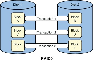
In this example, assume we have three transactions of two blocks each. So, Transaction1 needs to write two blocks to disk: Block A and Block B. Transaction2 needs to write Blocks C and D. Finally, Transaction3 needs to write Blocks E and F.

Each transaction takes only half the time to write to the RAID0 set as it would with a single disk because each of the two blocks are written simultaneously on Disk 1 and Disk 2, instead of writing the two blocks serially on a single disk. Of course, the downside is that if either drive fails, you lose the whole set, given that half of the data is on Disk 1 and the other half is on Disk 2.

RAID1

RAID1, called mirroring, is essentially a set of two disks in which every read and every write operation is performed on both disks simultaneously. Fault tolerance is improved because either disk can fail without crashing the array, allowing SQL Server to continue operating. The DBA or server administrator can then replace the failed drive without an emergency drill. RAID1 is essentially as fast as a single hard disk, but it is fault tolerant whenever a single disk in the array fails.

Figure 3.2 represents two disks in RAID1 configuration.

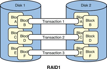
In this example, assume as before that we have three transactions of two blocks each, this time written to a RAID1 set. So, Transaction1 needs to write two blocks to disk: Block A and Block B. Transaction2 needs to write Blocks C and D. Finally, Transaction3 needs to write Blocks E and F.

Each transaction takes about the same to write to the RAID1 set as it would with a single disk because each of the two blocks are written sereally on Disk 1 and Disk 2, just like on a single disk. The big benefit here is that if either drive fails, you still have a full and complete copy of the data on both Disk 1 and Disk 2. And since there is no parity bit calculation, write speed is superior to that of RAID5.

RAID5

RAID5 is a group of at least three disks in which every read is striped across all the disks in the array. This means that read-centric IOPS are faster than with a single disk because the required data can be pulled from more than one disk simultaneously. Write performance, however, is slower than read performance on RAID5 because every write IOP also includes one additional parity write. This parity bit enables the array to reassemble any lost data should one of the drives in the array fail. That means a RAID5 can survive a single drive failure, but not more than one drive failure at a time.

It also means that RAID5 is good for read-heavy applications, but is not as good for write-heavy applications. RAID5 can be expanded beyond three disks, but is typically never bigger than seven disks because of the considerable time needed to reconstruct a failed drive from the parity bits written across all those other drives.

Figure 3.3 represents three disks in RAID5 configuration.

In this example, assume as before that we have three transactions of two blocks each, this time written to a RAID5 set. So, Transaction1 needs to write two blocks to disk: Block A and Block B. Transaction2 needs to write Blocks C and D. Finally, Transaction3 needs to write Blocks E and F.

The first difference you’ll notice is that RAID5 requires a minimum of three disks. Each transaction takes longer to write to the RAID5 set as it would with a single disk because each of the two blocks are written as a stripe across two of the disks while the third disk has a calculated parity bit written to it. The calculation and extra block write takes more time. A transaction that reads two blocks off of the RAID5 set would be faster than a single disk read, because the blocks are striped and could be read simultaneously. The benefit here is that if any single drive fails, you have enough information to recalculate the missing data using the parity blocks. The other benefit is that it is cheaper than other kinds of RAID sets.

But RAID5 has drawbacks too. First, write operations are a lot slower than on DASD or the other RAID configurations described here. Second, even though RAID5 provides inexpensive fault tolerance, should a drive fail, the process of calculating the values of the missing data from the parity blocks can be time consuming. So a full recovery, while easy to do, can be slower than on RAID1 or RAID10.

RAID10

RAID10 is also called RAID1+0. RAID10 is a group of at least four disks in which a RAID1 pair of disks are also striped, RAID0 style, to another pairs of RAID1 disks. This approach uses twice as many disks as RAID1. But it means that the array can sustain two failed drives simultaneously without crashing, as long as the failed disks are not in a single RAID1 pair. RAID10 has both fast read and write speeds, but is more expensive and consumes more space than RAID1 and RAID5.

Figure 3.4 represents four disks in RAID10 configuration.

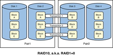
In this example, assume as before that we have three transactions of two blocks each, this time written to a RAID10 set. So, Transaction1 needs to write two blocks to disk: Block A and Block B. Transaction2 needs to write Blocks C and D. Finally, Transaction3 needs to write Blocks E and F.

The first difference you’ll notice is that RAID10 requires a minimum of four disks. Each transaction is faster to write to the RAID10 set as it would with a single disk because each of the two blocks are written as a stripe across each pair of mirrored disks. A transaction that reads two blocks off of the RAID 10 set would be much faster than a single disk read, because the blocks are striped and could be read simultaneously. So, both writes and reads are typically faster than any other option presented here.

In addition to speed of both read and write operations, RAID10 sets are more fault tolerant than any other configuration. That is because each mirrored pair within the RAID10 set can sustain a single disk failure, meaning that more than one disk can fail without causing the array to crash.

But RAID10 most obvious and dramatic drawback is the cost of requiring at least four disks. The disks themselves are costly, but they also consume plenty of space and energy as well. If you can afford them, RAID10 arrays are certainly the best option. But they constitute a much greater expense than DASD.

Disk Controllers and Host Bus Adapters (HBA)

Disks are typically configured and controlled using one of two popular standards: SCSI (pronounced “scuzzy”) and IDE/ATA (usually “A-T-A” for short). SCSI is by far the most popular standard for servers, whereas ATA (usually labeled as SATA) is the most popular standard for home and personal use. Servers using hard disks that adhere to these standards can be directly cabled to the disks, resulting in the acronym DASD, for Direct Attached Storage Device. DASD can also be cabled using standard network protocols like IP over Ethernet cable or Fibre Channel. Note that Fibre Channel and iSCSI are seen primarily on SANs.

Host bus adapters (HBAs) control the movement of data between the server motherboard and the hard disks. HBAs typically include performance options, such as a built-in cache, which can improve performance by buffering writes to the hard disk and then sending them in a burst.

NOTE

HBAs with write-cache controllers are not always safe for use with databases. How so? If a write-cache ever sustains a power failure, any write IOPS stored in the write-cache will vanish and be lost. As a precaution, many HBAs include a built-in battery backup. But the battery backup is not always be able to recharge or lose its ability to hold a charge without disabling the write-cache. Therefore, it’s important for DBAs to ensure that their HBA has a battery backup that automatically disables itself if the battery fails.

HBAs are important in storage and I/O discussions because it is possible, with enough active processes, to saturate a single HBA. For example, imagine a scheduled job attempts to back up all databases simultaneously on a SQL Server with multiple TBs of data while other I/O heavy operations were also processing. A situation like that could attempt to push through more I/O than the HBA can sustain. HBAs are also important because their firmware may need to be independently updated and maintained when faced with updates to Windows or other hardware components. Remember to stay apprised of vendor recommendations and updates when using high-end HBAs.

Network Attached Storage (NAS), Storage Area Networks (SAN), and Logical Units (LUN)

The Internet is full of information about digital storage. However, some of it is old, outdated, or simply not useful. With SQL Server and storage, consider Network Attached Storage (NAS) as one such area where DBAs should steer clear. Think of NAS servers as more of a file-and-print server technology, not suitable for SQL Server database files, transaction log files, or backup files. NAS may be useful in some Extract-Transform-Load (ETL) applications, but only when their use and potential failure won’t crash the production SQL Server database.

Storage Area Networks (SAN) are usually slightly slower than DASD, if only because they are more heavily used by a variety of applications than DASD. SAN is typically expensive and also has a degree of management overhead in that it should be set up, configured, and administrated only by a dedicated IT professional. But what it loses in speed, it makes up in flexibility, redundant components, and manageability.

For example, it is very easy to extend, reduce, or reconfigure storage on a SAN in Logical Units (LUNs) without stopping important Windows services, like SQL Server. These LUNs can be made available to Windows servers as if they were regular disk drives, when in fact they are usually RAID volumes or even just portions of RAID volumes. In fact, it is easy for SAN administrators to virtualize storage so that it can be quickly moved around on-the-fly.

This is great for SAN administrators, but it can be bad for DBAs if the storage the application has been depending upon is shared with another application in the enterprise. For example, it is possible to configure a large RAID10 volume as two LUNs. These two LUNs share the same underlying disks and, if both LUNS are busy, contend with one another for IOPS on the underlying RAID volume. It’s not good, but certainly a possibility.

Depending on the SAN in use, enormous amounts of cache may also be available to help speed I/O processing. These caches can also be quickly and easily configured (and reconfigured) by SAN administrators to better balance and tune applications that use the SAN.

Unfortunately, many if not most SAN administrators think about storage only as measured by volume, not IOPS or disk throughput. Consequently, it is up to DBAs to know how much I/O performance their applications need and to monitor I/O performance within SQL Server to ensure that they are achieving adequate I/O performance. Many a SAN administrator has been startled to find out that the SQL Server DBA is better informed about the I/O speed (or lack thereof) on the LUNs assigned to them than they are, usually due to a misconfigured setting somewhere on the SAN.

The bottom line for DBAs when administrating storage on a SAN is to follow the SAN vendor’s recommendations wherever possible, and then to monitor and performance tune the SQL Server instance as if the LUN(s) are normal disks.

Solid State Disks (SSD)

The new kids on the block for storage and I/O subsystems are several kinds of solid state disks (SSDs). SSDs are treated just like hard disks when configured, as individual devices or in RAID volumes. Because they are entirely electronic in nature, they offer significant savings in power consumption, speed, and resistance to damage from impact compared to hard disks. SSDs are becoming increasingly popular in the database administration community because they are remarkably faster than hard disks, especially for random I/O operations.

From a hardware perspective, a variety of different types of memory chips might be used within the SSD. But the two most common types of memory in SSDs are DRAM, which usually has volatile memory, and NAND flash memory, which is slower but nonvolatile. Volatile memory loses data when it loses power, whereas nonvolatile memory does not lose data when there is no power. When assessing flash memory-based SSDs, multilevel cell (MLC) flash memory is slower and less reliable than single-level cell (SLC) flash memory.

SSDs, however, have a few special considerations. First, the memory blocks within an SSD can be erased and rewritten a limited number of times. (DRAM-based SSD does not have this limitation.) Enterprise-quality flash drives work around this limitation by overprovisioning the amount of storage on the SSD through algorithms called wear leveling, thus ensuring that the SSD will last for the same duration as a similarly priced hard disk. Second, SSDs require a lot of free memory blocks to perform write operations. Whereas hard disks simply overwrite an unused sector, SSDs must clear out a previously written block using an algorithm called TRIM.

Finally, whereas SQL Server indexes residing on hard disks need frequent defragmentation, indexes residing on SSDs have no such requirement. Because all memory blocks on the SSD are only a few electrons away, all read access is pretty much the same speed whether the index pages are contiguous or not.

Now that you understand the most important aspects of storage hardware, let’s discuss the principles and management tasks that correlate the storage and I/O elements of SQL Server back to the system hardware.

The following “Notes from the Field” section introduces the one of the most commonly used methods of improving I/O performance: segregation of workload.

Notes from the Field: Segregating I/O for Better Performance and Reliability

One trick for improving storage performance, scalability, and fault tolerance is simply a process of segregating the I/O workload across the optimum number of I/O subcomponents-while balancing all those components against the cost of what the organization can afford. That is because hard disks have only one armature and read-write head per spinning disk, also known as a spindle.

Each spindle can only do one activity at a time. But we very often ask spindles to do contradictory work in a database application, such as performing a long serial read at the same time other users are asking it to do a lot of small, randomized writes. Any time a spindle is asked to do contradictory work, it simply takes much longer to finish the requests. On the other hand, when we ask disks to perform complementary work and segregate the contrary work off to a separate set of disks, performance improves dramatically.

For example, a SQL Server database will always have at least two files: a database file and a transaction log file. The I/O workload of the database file, many random reads and writes, stands in stark contrast to the I/O workload of the transaction log file, a series of sequential writes, one immediately after the other. Because the typical transactional database I/O workload is at odds with the transaction log I/O workload, the first step of segregation most DBAs perform is to put the database file(s) and the transaction log file on entirely separate disk, whether a single disk or RAID array or LUN on a SAN.

Similarly, if I/O performance is still underperforming, the DBA might then choose to segregate the tempdb workload onto an entirely separate disk array, because its workload is likely conflicting with or at least sapping the I/O performance of the main production database. As I/O needs grow, the DBA may choose a variety of other methods available to segregate I/O. SQL Server offers a variety of options to increase I/O performance entirely within SQL Server. However, DBAs also have a big bag of tricks, at the hardware level, available to improve I/O performance.

For example, when attempting to improve I/O performance within SQL Server, many DBAs will place all system databases (such as Master, MSDB, distribution, and the like) onto their own disk arrays, segregated away from the main production database(s). They may choose to add more files to the database’s filegroup and either explicitly place certain partitions, tables, and indexes onto the other files or allow SQL Server to automatically grow partitions, tables, and indexes onto the newly added file, thus further segregating I/O across more disk arrays. It is not uncommon to see very busy production databases with a lot of files, each on a different disk array. They might take the single busiest table in a database, which happens to generate 50% of the I/O on that instance, and split it into two partitions: one containing transactions under one week old (where most of the I/O occurs) and those over a week old, which are less frequently accessed as they age. The options abound.

On the hardware side of the equation, DBAs might reconfigure a specific drive (for instance, the F: drive) from a single disk to multiple disks in a RAID array with much higher I/O speed and capacity; for example, from 7,000 RPM disks to 15,000 RPM disks. They might upgrade a slower RAID 5 array to a faster RAID 10 array with a larger number of disks. They might increase the amount of read and write cache available on the hard disk controller(s) or SAN. They might add an additional hard disk controller to open more channels between the backplane and the I/O subsystem. In some cases, I/O problems are resolved by adding memory, when the I/O bottleneck is caused by constantly refreshing the buffer cache from disk. Again, a DBA can speed up the I/O subsystem in many ways.

But the fundamental principle applied in each of the previous examples is that the DBA is looking for an opportunity to take areas within SQL Server that are “bottlenecked” and segregate them to their own separate I/O component. Refer to and Chapter 14, “Performance Tuning and Troubleshooting SQL Server 2012,” and Chapter 15 for more details on monitoring SQL Server I/O and tuning performance storage and troubleshooting errors on SQL Server, respectively.

Designing and Administering Storage on SQL Server 2012

The following section is topical in approach. Rather than describe all the administrative functions and capabilities of a certain screen, such as the Database Settings page in the SSMS Object Explorer, this section provides a top-down view of the most important considerations when designing the storage for an instance of SQL Server 2012 and how to achieve maximum performance, scalability, and reliability.

This section begins with an overview of database files and their importance to overall I/O performance, in “Designing and Administering Database Files in SQL Server 2012,” followed by information on how to perform important step-by-step tasks and management operations. SQL Server storage is centered on databases, although a few settings are adjustable at the instance-level. So, great importance is placed on proper design and management of database files.

The next section, titled “Designing and Administering Filegroups in SQL Server 2012,” provides an overview of filegroups as well as details on important tasks. Prescriptive guidance also tells important ways to optimize the use of filegroups in SQL Server 2012.

Next, FILESTREAM functionality and administration are discussed, along with step-by-step tasks and management operations in the section “Designing for BLOB Storage.” This section also provides a brief introduction and overview to another supported method storage called Remote Blob Store (RBS).

Finally, an overview of partitioning details how and when to use partitions in SQL Server 2012, their most effective application, common step-by-step tasks, and common use-cases, such as a “sliding window” partition. Partitioning may be used for both tables and indexes, as detailed in the upcoming section “Designing and Administrating Partitions in SQL Server 2012.”

Designing and Administrating Database Files in SQL Server 2012

Whenever a database is created on an instance of SQL Server 2012, a minimum of two database files are required: one for the database file and one for the transaction log. By default, SQL Server will create a single database file and transaction log file on the same default destination disk. Under this configuration, the data file is called the Primary data file and has the .mdf file extension, by default. The log file has a file extension of .ldf, by default. When databases need more I/O performance, it’s typical to add more data files to the user database that needs added performance. These added data files are called Secondary files and typically use the .ndf file extension.

As mentioned in the earlier “Notes from the Field” section, adding multiple files to a database is an effective way to increase I/O performance, especially when those additional files are used to segregate and offload a portion of I/O. We will provide additional guidance on using multiple database files in the later section titled “Designing and Administrating Multiple Data Files.”

When you have an instance of SQL Server 2012 that does not have a high performance requirement, a single disk probably provides adequate performance. But in most cases, especially an important production database, optimal I/O performance is crucial to meeting the goals of the organization.

The following sections address important proscriptive guidance concerning data files. First, design tips and recommendations are provided for where on disk to place database files, as well as the optimal number of database files to use for a particular production database. Other guidance is provided to describe the I/O impact of certain database-level options.

Placing Data Files onto Disks

At this stage of the design process, imagine that you have a user database that has only one data file and one log file. Where those individual files are placed on the I/O subsystem can have an enormous impact on their overall performance, typically because they must share I/O with other files and executables stored on the same disks. So, if we can place the user data file(s) and log files onto separate disks, where is the best place to put them?

NOTE

Database files should reside only on RAID volumes to provide fault tolerance and availability while increasing performance. If cost is not an issue, data files and transaction logs should be placed on RAID1+0 volumes. RAID1+0 provides the best availability and performance because it combines mirroring with striping. However, if this is not a possibility due to budget, data files should be placed on RAID5 and transaction logs on RAID1. Refer to the earlier “Storage Hardware Overview” section in this chapter for more information.

When designing and segregating I/O by workload on SQL Server database files, there are certain predictable payoffs in terms of improved performance. When separating workload on to separate disks, it is implied that by “disks” we mean a single disk, a RAID1, -5, or -10 array, or a volume mount point on a SAN. The following list ranks the best payoff, in terms of providing improved I/O performance, for a transaction processing workload with a single major database:

1. Separate the user log file from all other user and system data files and log files. The server now has two disks:

• Disk A:\ is for randomized reads and writes. It houses the Windows OS files, the SQL Server executables, the SQL Server system databases, and the production database file(s).
• Disk B:\ is solely for serial writes (and very occasionally for writes) of the user database log file. This single change can often provide a 30% or greater improvement in I/O performance compared to a system where all data files and log files are on the same disk.

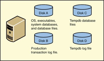
Figure 3.5 shows what this configuration might look like.

1. Separate tempdb, both data file and log file onto a separate disk. Even better is to put the data file(s) and the log file onto their own disks. The server now has three or four disks:

• Disk A:\ is for randomized reads and writes. It houses the Windows OS files, the SQL Server executables, the SQL Server system databases, and the user database file(s).
• Disk B:\ is solely for serial reads and writes of the user database log file.
• Disk C:\ for tempd data file(s) and log file. Separating tempdb onto its own disk provides varying amounts of improvement to I/O performance, but it is often in the mid-teens, with 14-17% improvement common for OLTP workloads.
• Optionally, Disk D:\ to separate the tempdb transaction log file from the tempdb database file.

Figure 3.6 shows an example of intermediate file placement for OLTP workloads.

1. Separate user data file(s) onto their own disk(s). Usually, one disk is sufficient for many user data files, because they all have a randomized read-write workload. If there are multiple user databases of high importance, make sure to separate the log files of other user databases, in order of business, onto their own disks. The server now has many disks, with an additional disk for the important user data file and, where needed, many disks for log files of the user databases on the server:

• Disk A:\ is for randomized reads and writes. It houses the Windows OS files, the SQL Server executables, and the SQL Server system databases.
• Disk B:\ is solely for serial reads and writes of the user database log file.
• Disk C:\ is for tempd data file(s) and log file.
• Disk E:\ is for randomized reads and writes for all the user database files.
• Drive F:\ and greater are for the log files of other important user databases, one drive per log file.

Figure 3.7 shows and example of advanced file placement for OLTP workloads.

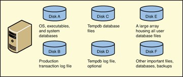
1. Repeat step 3 as needed to further segregate database files and transaction log files whose activity creates contention on the I/O subsystem. And remember-the figures only illustrate the concept of a logical disk. So, Disk E in Figure 3.7 might easily be a RAID10 array containing twelve actual physical hard disks.

Utilizing Multiple Data Files

As mentioned earlier, SQL Server defaults to the creation of a single primary data file and a single primary log file when creating a new database. The log file contains the information needed to make transactions and databases fully recoverable. Because its I/O workload is serial, writing one transaction after the next, the disk read-write head rarely moves. In fact, we don’t want it to move. Also, for this reason, adding additional files to a transaction log almost never improves performance. Conversely, data files contain the tables (along with the data they contain), indexes, views, constraints, stored procedures, and so on. Naturally, if the data files reside on segregated disks, I/O performance improves because the data files no longer contend with one another for the I/O of that specific disk.

Less well known, though, is that SQL Server is able to provide better I/O performance when you add secondary data files to a database, even when the secondary data files are on the same disk, because the Database Engine can use multiple I/O threads on a database that has multiple data files. The general rule for this technique is to create one data file for every two to four logical processors available on the server. So, a server with a single one-core CPU can’t really take advantage of this technique. If a server had two four-core CPUs, for a total of eight logical CPUs, an important user database might do well to have four data files.

The newer and faster the CPU, the higher the ratio to use. A brand-new server with two four-core CPUs might do best with just two data files. Also note that this technique offers improving performance with more data files, but it does plateau at either 4, 8, or in rare cases 16 data files. Thus, a commodity server might show improving performance on user databases with two and four data files, but stops showing any improvement using more than four data files. Your mileage may vary, so be sure to test any changes in a nonproduction environment before implementing them.

Sizing Multiple Data Files

Suppose we have a new database application, called BossData, coming online that is a very important production application. It is the only production database on the server, and according to the guidance provided earlier, we have configured the disks and database files like this:

1. Drive C:\ is a RAID1 pair of disks acting as the boot drive housing the Windows Server OS, the SQL Server executables, and the system databases of Master, MSDB, and Model.
2. Drive D:\ is the DVD drive.
3. Drive E:\ is a RAID1 pair of high-speed SSDs housing tempdb data files and the log file.
4. DRIVE F:\ in RAID10 configuration with lots of disks houses the random I/O workload of the eight BossData data files: one primary file and seven secondary files.
5. DRIVE G:\ is a RAID1 pair of disks housing the BossData log file.

Most of the time, BossData has fantastic I/O performance. However, it occasionally slows down for no immediately evident reason. Why would that be?

As it turns out, the size of multiple data files is also important. Whenever a database has one file larger than another, SQL Server will send more I/O to the large file because of an algorithm called round-robin, proportional fill. “Round-robin” means that SQL Server will send I/O to one data file at a time, one right after the other. So for the BossData database, the SQL Server Database Engine would send one I/O first to the primary data file, the next I/O would go to the first secondary data file in line, the next I/O to the next secondary data file, and so on. So far, so good.

However, the “proportional fill” part of the algorithm means that SQL Server will focus its I/Os on each data file in turn until it is as full, in proportion, to all the other data files. So, if all but two of the data files in the BossData database are 50Gb, but two are 200Gb, SQL Server would send four times as many I/Os to the two bigger data files in an effort to keep them as proportionately full as all the others.

In a situation where BossData needs a total of 800Gb of storage, it would be much better to have eight 100Gb data files than to have six 50Gb data files and two 200Gb data files.

TIP

To see the latency of all of the data files, the log file, and the disks they reside on, use this query:

SELECT physical_name AS drive,
  CAST(SUM(io_stall_read_ms) / (1.0 + SUM(num_of_reads))
AS NUMERIC(10, 1)) AS 'Avg Read Latency/ms',
  CAST(SUM(io_stall_write_ms) / (1.0 +
SUM(num_of_writes)) AS NUMERIC(10, 1)) AS 'Avg Write
Latency/ms',
  CAST((SUM(io_stall)) / (1.0 + SUM(num_of_reads +
num_of_writes)) AS NUMERIC(10, 1)) AS 'Avg Disk
Latency/ms'
FROM sys.dm_io_virtual_file_stats(NULL, NULL) AS d
  JOIN sys.master_files AS m
       ON m.database_id = d.database_id
       AND m.file_id = d.file_id
GROUP BY physical_name
ORDER BY physical_name DESC;

Remember, Microsoft’s recommendation is that data file latency should not exceed 20ms, and log file latency should not exceed 10ms. But in practice, a latency that is twice as high as the recommendations is often acceptable to most users.

Autogrowth and I/O Performance

When you’re allocating space for the first time to both data files and log files, it is a best practice to plan for future I/O and storage needs, which is also known as capacity planning.

In this situation, estimate the amount of space required not only for operating the database in the near future, but estimate its total storage needs well into the future. After you’ve arrived at the amount of I/O and storage needed at a reasonable point in the future, say one year hence, you should preallocate the specific amount of disk space and I/O capacity from the beginning.

Over-relying on the default autogrowth features causes two significant problems. First, growing a data file causes database operations to slow down while the new space is allocated and can lead to data files with widely varying sizes for a single database. (Refer to the earlier section “Sizing Multiple Data Files.”) Growing a log file causes write activity to stop until the new space is allocated. Second, constantly growing the data and log files typically leads to more logical fragmentation within the database and, in turn, performance degradation.

Most experienced DBAs will also set the autogrow settings sufficiently high to avoid frequent autogrowths. For example, data file autogrow defaults to a meager 25Mb, which is certainly a very small amount of space for a busy OLTP database. It is recommended to set these autogrow values to a considerable percentage size of the file expected at the one-year mark. So, for a database with 100Gb data file and 25GB log file expected at the one-year mark, you might set the autogrowth values to 10Gb and 2.5Gb, respectively.

NOTE

We still recommend leaving the Autogrowth option enabled. You certainly do not want to ever have a data file and especially a log file run out of space during regular daily use. However, our recommendation is that you do not rely on the Autogrowth option to ensure the data files and log files have enough open space. Preallocating the necessary space is a much better approach.

Additionally, log files that have been subjected to many tiny, incremental autogrowths have been shown to underperform compared to log files with fewer, larger file growths. This phenomena occurs because each time the log file is grown, SQL Server creates a new VLF, or virtual log file. The VLFs connect to one another using pointers to show SQL Server where one VLF ends and the next begins. This chaining works seamlessly behind the scenes. But it’s simple common sense that the more often SQL Server has to read the VLF chaining metadata, the more overhead is incurred. So a 20Gb log file containing four VLFs of 5Gb each will outperform the same 20Gb log file containing 2000 VLFs.

Configuring Autogrowth on a Database File

To configure autogrowth on a database file (as shown in Figure 3.8), follow these steps:

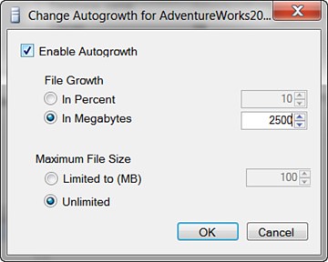
1. From within the File page on the Database Properties dialog box, click the ellipsis button located in the Autogrowth column on a desired database file to configure it.
2. In the Change Autogrowth dialog box, configure the File Growth and Maximum File Size settings and click OK.
3. Click OK in the Database Properties dialog box to complete the task.

You can alternately use the following Transact-SQL syntax to modify the Autogrowth settings for a database file based on a growth rate of 10Gb and an unlimited maximum file size:

USE [master]
GO
ALTER DATABASE [AdventureWorks2012]
MODIFY FILE ( NAME = N'AdventureWorks2012_Data',
MAXSIZE = UNLIMITED , FILEGROWTH = 10240KB
)
GO

TIP

The prevailing best practice for autogrowth is to use an absolute number, such as 100Mb, rather than a percentage, because most DBAs prefer a very predictable growth rate on their data and transaction log files.

Data File Initialization

Anytime SQL Server has to initialize a data or log file, it overwrites any residual data on the disk sectors that might be hanging around because of previously deleted files. This process fills the files with zeros and occurs whenever SQL Server creates a database, adds files to a database, expands the size of an existing log or data file through autogrow or a manual growth process, or due to a database or filegroup restore. This isn’t a particularly time-consuming operation unless the files involved are large, such as over 100Gbs. But when the files are large, file initialization can take quite a long time.

It is possible to avoid full file initialization on data files through a technique call instant file initialization. Instead of writing the entire file to zeros, SQL Server will overwrite any existing data as new data is written to the file when instant file initialization is enabled. Instant file initialization does not work on log files, nor on databases where transparent data encryption is enabled.

SQL Server will use instant file initialization whenever it can, provided the SQL Server service account has SE_MANAGE_VOLUME_NAME privileges. This is a Windows-level permission granted to members of the Windows Administrator group and to users with the Perform Volume Maintenance Task security policy.

For more information, refer to the SQL Server Books Online documentation.

Shrinking Databases, Files, and I/O Performance

The Shrink Database task reduces the physical database and log files to a specific size. This operation removes excess space in the database based on a percentage value. In addition, you can enter thresholds in megabytes, indicating the amount of shrinkage that needs to take place when the database reaches a certain size and the amount of free space that must remain after the excess space is removed. Free space can be retained in the database or released back to the operating system.

It is a best practice not to shrink the database. First, when shrinking the database, SQL Server moves full pages at the end of data file(s) to the first open space it can find at the beginning of the file, allowing the end of the files to be truncated and the file to be shrunk. This process can increase the log file size because all moves are logged. Second, if the database is heavily used and there are many inserts, the data files may have to grow again.

SQL 2005 and later addresses slow autogrowth with instant file initialization; therefore, the growth process is not as slow as it was in the past. However, sometimes autogrow does not catch up with the space requirements, causing a performance degradation. Finally, simply shrinking the database leads to excessive fragmentation. If you absolutely must shrink the database, you should do it manually when the server is not being heavily utilized.

You can shrink a database by right-clicking a database and selecting Tasks, Shrink, and then Database or File.

Alternatively, you can use Transact-SQL to shrink a database or file. The following Transact=SQL syntax shrinks the AdventureWorks2012 database, returns freed space to the operating system, and allows for 15% of free space to remain after the shrink:

USE [AdventureWorks2012]
GO
DBCC SHRINKDATABASE(N'AdventureWorks2012', 15, TRUNCATEONLY)
GO

NOTE

Although it is possible to shrink a log file, SQL Server is not able to shrink the log file past the oldest, active transaction. For example, imagine a 10Gb transaction log that has been growing at an alarming rate with the potential to fill up the disk soon. If the last open transaction was written to the log file at the 7Gb mark, even if the space prior to that mark is essentially unused, the shrink process will not be able to shrink the log file to anything smaller than 7Gb. To see if there are any open transactions in a given database, use the Transact-SQL command DBCC OPENTRAN.

TIP

It is best practice not to select the option to shrink the database. First, when shrinking the database, SQL Server moves pages toward the beginning of the file, allowing the end of the files to be shrunk. This process can increase the transaction log size because all moves are logged. Second, if the database is heavily used and there are many inserts, the database files will have to grow again. SQL 2005 and above addresses slow autogrowth with instant file initialization; therefore, the growth process is not as slow as it was in the past. However, sometimes autogrow does not catch up with the space requirements, causing performance degradation. Finally, constant shrinking and growing of the database leads to excessive fragmentation. If you need to shrink the database size, you should do it manually when the server is not being heavily utilized.

Administering Database Files

The Database Properties dialog box is where you manage the configuration options and values of a user or system database. You can execute additional tasks from within these pages, such as database mirroring and transaction log shipping. The configuration pages in the Database Properties dialog box that affect I/O performance include the following:

• Files
• Filegroups
• Options
• Change Tracking

The upcoming sections describe each page and setting in its entirety. To invoke the Database Properties dialog box, perform the following steps:

1. Choose Start, All Programs, Microsoft SQL Server 2012, SQL Server Management Studio.
2. In Object Explorer, first connect to the Database Engine, expand the desired instance, and then expand the Databases folder.
3. Select a desired database, such as AdventureWorks2012, right-click, and select Properties. The Database Properties dialog box is displayed.

Administering the Database Properties Files Page

The second Database Properties page is called Files. Here you can change the owner of the database, enable full-text indexing, and manage the database files, as shown in Figure 3.9.

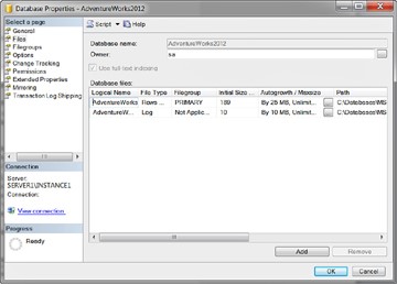
Administrating Database Files

Use the Files page to configure settings pertaining to database files and transaction logs. You will spend time working in the Files page when initially rolling out a database and conducting capacity planning. Following are the settings you’ll see:

• Data and Log File Types-A SQL Server 2012 database is composed of two types of files: data and log. Each database has at least one data file and one log file. When you’re scaling a database, it is possible to create more than one data and one log file. If multiple data files exist, the first data file in the database has the extension *.mdf and subsequent data files maintain the extension *.ndf. In addition, all log files use the extension *.ldf.
• Filegroups-When you’re working with multiple data files, it is possible to create filegroups. A filegroup allows you to logically group database objects and files together. The default filegroup, known as the Primary Filegroup, maintains all the system tables and data files not assigned to other filegroups. Subsequent filegroups need to be created and named explicitly.
• Initial Size in MB-This setting indicates the preliminary size of a database or transaction log file. You can increase the size of a file by modifying this value to a higher number in megabytes.

Increasing Initial Size of a Database File

Perform the following steps to increase the data file for the AdventureWorks2012 database using SSMS:

1. In Object Explorer, right-click the AdventureWorks2012 database and select Properties.
2. Select the Files page in the Database Properties dialog box.
3. Enter the new numerical value for the desired file size in the Initial Size (MB) column for a data or log file and click OK.

Other Database Options That Affect I/O Performance

Keep in mind that many other database options can have a profound, if not at least a nominal, impact on I/O performance. To look at these options, right-click the database name in the SSMS Object Explorer, and then select Properties. The Database Properties page appears, allowing you to select Options or Change Tracking. A few things on the Options and Change Tracking tabs to keep in mind include the following:

• Options: Recovery Model-SQL Server offers three recovery models: Simple, Bulk Logged, and Full. These settings can have a huge impact on how much logging, and thus I/O, is incurred on the log file. Refer to Chapter 6, “Backing Up and Restoring SQL Server 2012 Databases,” for more information on backup settings.
• Options: Auto-SQL Server can be set to automatically create and automatically update index statistics. Keep in mind that, although typically a nominal hit on I/O, these processes incur overhead and are unpredictable as to when they may be invoked. Consequently, many DBAs use automated SQL Agent jobs to routinely create and update statistics on very high-performance systems to avoid contention for I/O resources.
• Options: State: Read-Only-Although not frequent for OLTP systems, placing a database into the read-only state enormously reduces the locking and I/O on that database. For high reporting systems, some DBAs place the database into the read-only state during regular working hours, and then place the database into read-write state to update and load data.
• Options: State: Encryption-Transparent data encryption adds a nominal amount of added I/O overhead.
• Change Tracking-Options within SQL Server that increase the amount of system auditing, such as change tracking and change data capture, significantly increase the overall system I/O because SQL Server must record all the auditing information showing the system activity.

Designing and Administering Filegroups in SQL Server 2012

Filegroups are used to house data files. Log files are never housed in filegroups. Every database has a primary filegroup, and additional secondary filegroups may be created at any time. The primary filegroup is also the default filegroup, although the default file group can be changed after the fact. Whenever a table or index is created, it will be allocated to the default filegroup unless another filegroup is specified.

Filegroups are typically used to place tables and indexes into groups and, frequently, onto specific disks. Filegroups can be used to stripe data files across multiple disks in situations where the server does not have RAID available to it. (However, placing data and log files directly on RAID is a superior solution using filegroups to stripe data and log files.) Filegroups are also used as the logical container for special purpose data management features like partitions and FILESTREAM, both discussed later in this chapter. But they provide other benefits as well. For example, it is possible to back up and recover individual filegroups. (Refer to Chapter 6 for more information on recovering a specific filegroup.)

To perform standard administrative tasks on a filegroup, read the following sections.

Creating Additional Filegroups for a Database

Perform the following steps to create a new filegroup and files using the AdventureWorks2012 database with both SSMS and Transact-SQL:

1. In Object Explorer, right-click the AdventureWorks2012 database and select Properties.
2. Select the Filegroups page in the Database Properties dialog box.
3. Click the Add button to create a new filegroup.
4. When a new row appears, enter the name of the new filegroup and enable the option Default.

Alternately, you may create a new filegroup as a set of adding a new file to a database, as shown in Figure 3.10. In this case, perform the following steps:

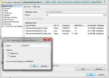
1. In Object Explorer, right-click the AdventureWorks2012 database and select Properties.
2. Select the Files page in the Database Properties dialog box.
3. Click the Add button to create a new file. Enter the name of the new file in the Logical Name field.
4. Click in the Filegroup field and select <new filegroup>.
5. When the New Filegroup page appears, enter the name of the new filegroup, specify any important options, and then click OK.

Alternatively, you can use the following Transact-SQL script to create the new filegroup for the AdventureWorks2012 database:

USE [master]
GO
ALTER DATABASE [AdventureWorks2012] ADD FILEGROUP
[SecondFileGroup]
GO

To finish reading this article click here: http://www.informit.com/articles/article.aspx?p=1946159