


Artificial intelligence (AI) is one of the hottest topics these days. With the advancement in hardware technologies, it's now possible to do things that were once deemed impossible. Autonomous driving is no longer a dream, and fully autonomous driving is fast becoming a reality. A subset of AI is machine learning, and deep learning itself is a subset of machine learning. In my earlier two articles in CODE Magazine (September/October 20017 and November/December 2017), I talked about machine learning using the Microsoft Azure Machine Learning Studio, as well as how to perform machine learning using the Scikit-learn library. In this article, let's turn our attention to one of the most exciting (if not seemingly magical) topics in AI; Deep Learning.
What is Deep Learning?
If you're familiar with machine learning and its associated algorithms (linear regression, logistic regression, Support Vector Machine, K-Nearest Neighbors, K-Means, etc.), you're no stranger to the various steps needed to feed your data to the algorithms in order to train the model to perform predictions. Predictably, you need to perform the following steps:
- Data cleansing
- Data visualization
- Features selection
- Splitting dataset for training and testing
- Evaluating different algorithms
In short, machine learning requires feature engineering. You need to structure your data first and then follow a standard procedure to solve the problem; break the problem into smaller parts and then solve each of them and combine them to get the required result.
Wouldn't it be great if there were a much easier way to train a model such that you just need to feed your data to an algorithm and it auto-magically establishes the relationship between your input and output? Turns out that there's really such a magical algorithm: that's deep learning.
Before I dive into how deep learning works, it's essential to define what deep learning is. Deep learning is a machine learning method that takes an input X and predicts an output Y. It does this by taking a given set of inputs and their associated outputs, and it tries to minimize the difference between the prediction and expected output. In short, deep learning learns the relationships between the input and output. Once the learning is done, it will be able to predict new output based on your input.
Understanding Neural Networks
To understand deep learning, you need to understand Artificial Neural Networks (ANN).
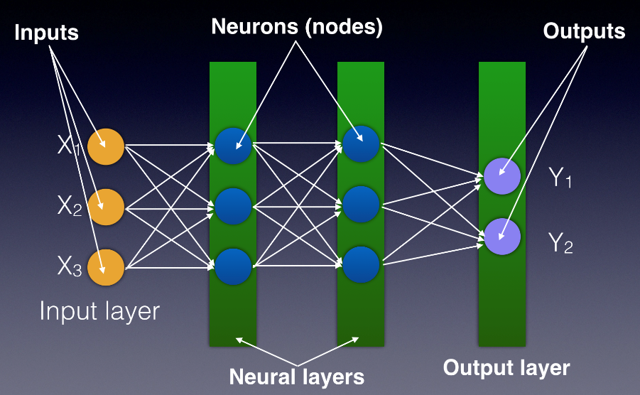
Figure 1 shows a neural network consisting of the following components:
- Input layer: Your data goes into the neural network through the input layer.
- Hidden/neural layers: The hidden layers contain neurons (also known as nodes). Typically, in a neural network, there are one or more hidden layers.
- Output layer: The output of the neural network is the predictions that you're trying to get out of the network.
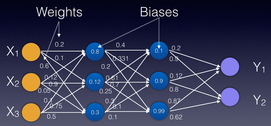
Each node in a layer connects to all the other nodes in the next layer. Each connection between nodes has a value known as the weight, and each node has a value known as the bias (see Figure 2). Initially, weights and biases are randomly assigned to each connection and node. The key role of a neural network is to find the ideal set of weights and biases that best describes the relationships between the input and the output.
The key role of a neural network is to find the ideal set of weights and biases that best describes the relationships between the input and the output.
What does this mean? Let's take a look at an example. Using the classic example of the Titanic dataset, consider a specific row where the age is 18, cabin class is first class (1), and number of siblings is 1. This will serve as the input for the neural network. This particular passenger didn't survive the disaster, and so the output is 0. When the neural network is trained using the Titanic dataset, the neural network has a set of weights and biases that allow you to predict the probability of survival of another new passenger. How the network is trained is the magic behind deep learning, and this is what I'll dive deeper into later in this article.
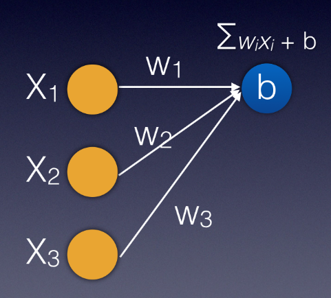
With the network trained (with the weights and biases derived), you can supply new passenger details through the input layer. Starting with the inputs at the input layer, the value of each node is multiplied with the weight for the particular connection and added to the biases at the next node. Figure 3 summarizes the formula for calculating the value at the next node.
Activation Function
After the value of the node is calculated, the value is passed into a function known as the activation function. The role of an activation function is to help you normalize (control) the output of a neural network. Let's see how an activation function works before I discuss why you need one.
The Activation Function is also known as the step function.
There are a few types of activation functions; here are some common types:
- Binary step activation function
- Linear activation functions
- Non-linear activation functions
Binary Step Function
The output of the binary step activation function looks like Figure 4.
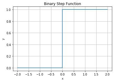
A binary activation function is a threshold-based activation function; if the input value is above or below a certain threshold, it outputs a value of 1 or 0, respectively.
An easy way to imagine the binary step function is to use this analogy. Suppose you place your hand on the kettle. Your hands will be on the kettle as long as the temperature on the kettle is below your tolerance threshold. The moment the water in the kettle starts to boil and reaches a temperature that's too hot for you to handle, you immediately remove your hands from the kettle. In this example, the temperature of the kettle is the input and the placement of your hand is the output.
Linear Activation Function
The output of the linear activation function is not limited to any range. Figure 5 shows the graph for a linear function.
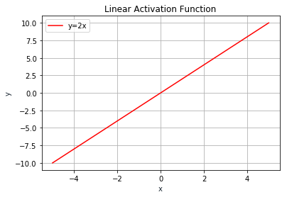
The linear activation function is of the form y = cx. The derivative of this function is a constant: dy/dx = c and has no relation to the input (x). When there's an error in prediction, you wouldn't be able to understand how changes to x affect the predicted output. A neural network with a linear activation function is simply a linear regression model. It has limited power and ability to handle complexity varying parameters of input data. Linear activation function is usually used at the output layer, when you need to predict a range of values.
A neural network with a linear activation function is simply a linear regression model.
Non-Linear Activation Function
There are several non-linear activation functions. The Sigmoid (logistic) activation function is an example of a non-linear activation function. The output of the Sigmoid function lies in (0,1).
The formula for the Sigmoid activation function is as shown in Figure 6.

Figure 7 shows the graph of the Sigmoid activation function.
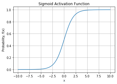
The Sigmoid activation function is useful for models where you have to predict the probability as an output. It's commonly used at the output layer to determine the probability of a prediction. For example, if the neural network outputs multiple answers (such as the detection of various objects in an image), you can use the Sigmoid activation function to calculate the probability of each prediction, such as:
- Dog; 0.8
- Cat: 0.4
- Guinea Pig: 0.1
Note that the sum of the three outputs above need not be equal to one. In cases where your neural network outputs a probability distribution (such as the probabilities of a person being male, female, or unknown), you need to use a Softmax activation function. Figure 8 shows the formula for the Softmax function.
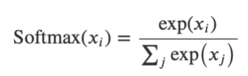
Figure 9 shows the graph of the Softmax activation function taking in an input list of [0.4, 3.0, 2.2]. The value on the y-axis is the output of the Softmax function: [0.04874866 0.65633915 0.29491219].
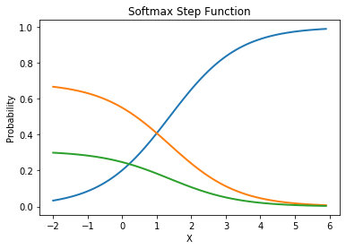
When used on the example of predicting the gender of a person in a picture, this translates to:
- Male: 0.04874866
- Female: 0.65633915
- Unknown: 0.29491219
Note that all probabilities add up to 1.
Another commonly used activation function is known as the Hyperbolic Tangent activation function (commonly written as Tanh). Figure 10 shows the Tanh activation function compared to the Sigmoid activation function.
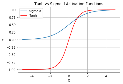
Observe that the output of the Tanh activation function lies in (-1,1). The Tanh activation function works very much like the logistic Sigmoid activation function. Its key advantage is that the negative input will be mapped strongly negative and the zero inputs will be mapped near zero. Tanh is mainly used for two-class classifications.
Besides the Tanh and Sigmoid activation functions, another non-linear activation function that's most used in the world of machine learning at this moment is known as the Rectified Linear Unit (or commonly known as ReLU).
Figure 11 shows what the ReLU activation function looks like. It's half rectified (from the bottom). R(x) is zero when X is less than zero and R(x) is equal to X when X is above or equal to zero. Observe that its output lies in [0, infinity).
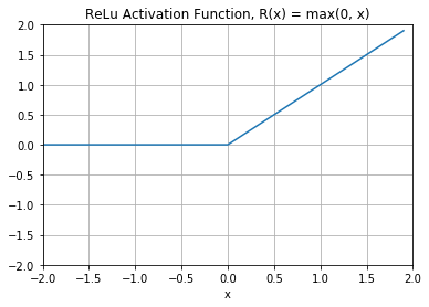
One issue with ReLU is that any negative input given to the ReLU activation function turns the value into zero immediately in the graph, which, in turn, affects the resulting graph by not mapping the negative values appropriately. This decreases the ability of the model to fit or train from the data properly.
To solve the dying ReLU problem, researchers came out with a novel solution named Leaky ReLU. Figure 12 shows what the Leaky ReLU activation looks like.
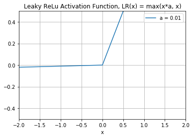
The formula for Leaky ReLU is:
LR(x) = max(x*a, x)
As you can see from the figure, the “leak” on the left chart of the graph helps to increase the range of the ReLU function. Usually, the value of a is 0.01 or so. When a is not 0.01, it's called Randomized ReLU. The range of the Leaky ReLU is (-infinity to infinity).
Loss Functions
In the previous section, you learned that after the value of each node is calculated, it's passed to an activation function, whose output is then passed to the next neuron for calculation.
After the neural network passes its inputs all the way to its outputs, the network evaluates how good its prediction was (relative to the expected output) through something called a loss function (also known as cost function). The Mean Squared Error (MSE), is one such function.
Figure 13 shows the formula for calculating the MSE, where Yi is the expected output, Y^I is the predicted output, and n is the number of samples.
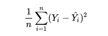
When training a neural network, aim to minimize the loss function so as to minimize the errors of your model.
Cross Entropy
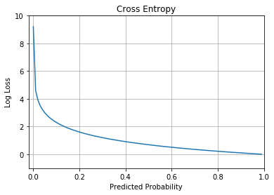
Besides MSE (which is often used for regression), you can also use the cross-entropy loss function. The cross-entropy loss (also known as log loss) function is shown in Figure 14.
Cross entropy can be applied to classification problems. In particular, if you're solving a:
- Binary classification problem, use binary cross entropy
- Multi-class classification problem, use categorical cross entropy
The formula for binary cross entropy is:
-(??log(??)+(1-??)log(1-??))
In this example, y is the actual output and P is the predicted probability.
Cross-entropy loss increases when the predicted probability deviates from the actual label. For example, if the actual result is 1 and the predicted probability is 0.01, the log loss is much higher than if the predicted probability is closer to 1. A perfect model would have a log loss of 0.
For categorical cross entropy, the formula is:
 ??
-? ????,??log(????,??)
 ??=1
In this example, M is the number of classes, ????,?? is the result (0 or 1) if class label c is the correct classification for observation ??, ????,?? is the predicted probability observation o of class c. Categorical cross entropy is also known as the softmax loss.
Backpropagation Using Optimizer
As described in the previous section, using a loss function allows you to know how much your prediction has deviated from the expected output. The aim is to minimize the value of the loss function. So how do you do that? You need to traverse back up the neural network to update the weights and biases so that your new predicted output will result in a lower loss. But with so many weights and biases, how do you efficiently adjust the weights and biases so that you can achieve minimal loss?
You can do this via a technique known as backpropagation. Using backpropagation, the network backtracks through all its layers to update the weights and biases of every node in the opposite direction of the loss function. Each iteration of back propagation should result in a smaller loss function than before. The continuous updates of the weights and biases of the network should ultimately turn it into a precise model that maps the relationship between inputs and expected outputs.
In the next section, I'll walk you through how backpropagation works by using a simple example.
Expressing the Loss Function as a Function of Weights
Consider Figure 15. Here, you have an input represented as an input vector (x). The input vector is multiplied with the weights (W) to produce the computed target (y_pred). The expected target is y.
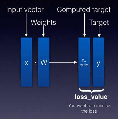
The loss value is the difference between the computed target and the target. The loss value can be expressed as a function of W, like this:
Loss_value = f(W)
Your aim is to reduce the loss value, i.e., reduce the value of f(W).
Understanding Derivatives (Gradients)
Before you understand how backpropagation works, it's useful to revisit some basic calculus. Figure 16 shows the loss function f(W) plotted as a curve.
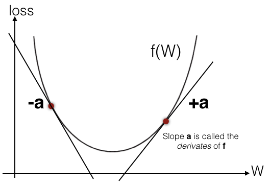
The slope (gradient) on any particular point on the curve is the derivative of the function: df(W)/dW. In the figure, a is the gradient of a point on the slope. You can observe the following:
- If a is positive (+), this means a small increase in W will result in an increase of f(W).
- If a is negative (-), this means a small increase in W will result in a decrease of f(W).
- The absolute value of a tells you the magnitude of change.
- The derivative completely describes how f(W) evolves as you change W.
Hence, you can conclude that for a particular value of W, the derivative of the loss function f(W) will tell how much the loss value is increasing or decreasing. More importantly, if you want to reduce the value of f(W), you just need to move W a little in the opposite direction from its derivative. You will see the importance of this statement in a short while.
If you want to reduce the value of the loss function f(W), you just need to move W a little in the opposite direction from its derivative.
A Walkthrough of Gradient Descent
To understand how backpropagation works, let's walk through an example using a popular backpropagation algorithm: gradient descent.
Gradient descent is known as an optimizer algorithm.
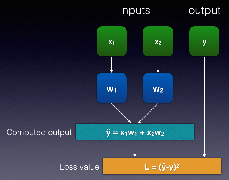
First, assume that you have a dataset with two inputs, x1 and x2, and an output y. Suppose you have a very simple neural network, as shown in Figure 17. Note that, for simplicity, I have omitted the biases in this illustration.
Let's try to plug in the first row of the dataset. Suppose you have inputs x1 = 4, x2 = 5, and y = 6. For the initial iteration of the training process, you initialize the weights with some random values, say w1 = -0.234 and w2 = 0.675. You can now start to calculate the value of y^ as well as the loss value (see Figure 18).
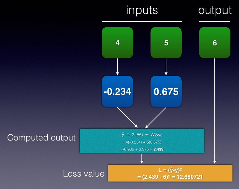
The loss value of the first row is 12.680721. The aim is to modify the weights so that in the next iteration, the loss value can be reduced. How much should you change the weights? Before you do that, let's look at some formulas. You know the following:
y^ = x1w1 + x2w2
L = (y^-y)2
   = y^2 - 2yy^ + y2
Let's take the partial differentials of the above formulas with respect to the various variables:
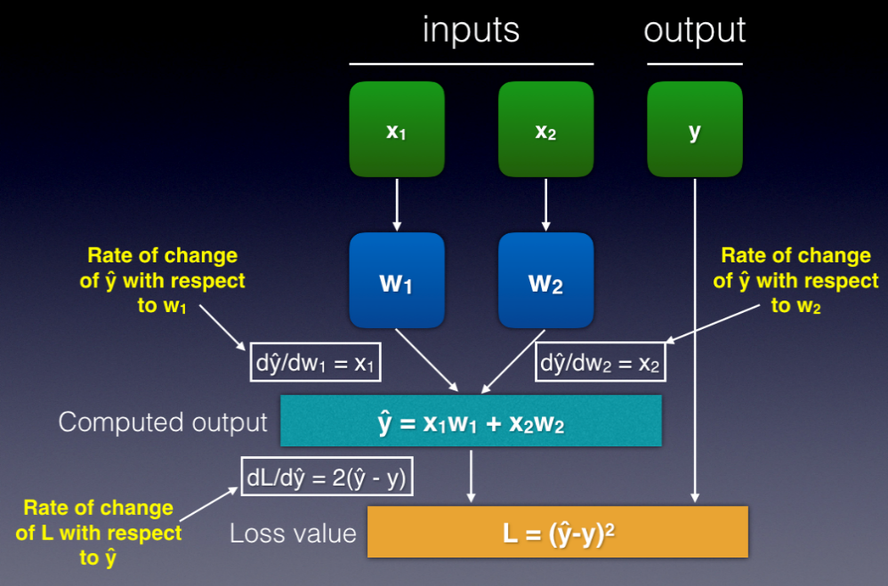
dL/dy^ = 2y^ - 2y
      = 2(y^ - y)
dy^/dw1 = x1
dy^/dw2 = x2
So dL/dy^ represents the rate of change of L with respect to y^. Likewise, dy^/dw1 represents the rate of change of y^ with respect to w1, and so on. You can now plug in the formulas to the network, as shown in Figure 19.
Based on the formulas, you're now ready to update the weights based on the following formula:
w1' = w1 - ?(dL/dw1)
Where:
w1'is the value of w1 after the updatew1is the current value of w1?is the learning rate = 0.05; usually a value from 0 to 1dL/dw1is the rate of change of L with respect to w1
Observe the minus sign in the equation. Remember, earlier on I mentioned that if you want to reduce the value of the loss function (f(W)), you just need to move W a little in the opposite direction from its derivative.
To find dL/dw1, it can be expressed as:
dL/dw1 = dL/dy^ * dy^/dw1
And from the previous equations, you know that:
dL/dy^ = 2(y^ - y)
dy^/dw1 = x1
Hence, dL/dw1 can be expressed in terms of y^, y, and x1, like this:
dL/dw1 = 2(y^ - y) * x1
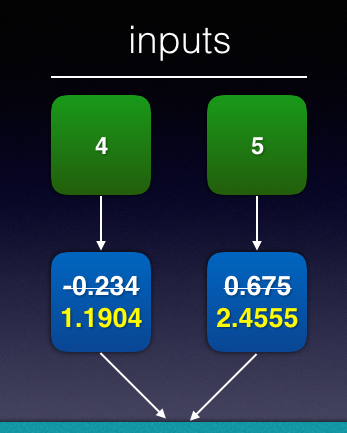
With x1 = 4, w1 = -0.234, y = 6, ? = 0.05, y^ = 2.439 (see Figure 18):
w1' = w1 - ?(dL/dw1)
    = -0.234 – 0.05(2(2.439 - 6) * 4)
    = 1.1904
Similarly, for w2', the formula is:
w2' = w2 - ?(dL/dw2)
dL/dw2 = dL/dy^ * dy^/dw2
dL/dy^ = 2(y^ - y)
dy^/dw2 = x2
With x2 = 5, w2 = 0.675, y = 6, ? = 0.05, y^ = 2.439 (see Figure 18):
w2' = w2 - ?(dL/dw2)
    = 0.675 – 0.05(2(2.439 - 6) * 5)
    = 2.4555
You can now update the value for w1 and w2 (see Figure 20).
That's the end of the first row in your dataset. You need to repeat the steps described above for the rest of the rows in your dataset. After going through all the rows in your dataset, that's one epoch completed. In order for the loss to converge, you need to perform multiple epochs to update the weights and biases in each iteration. At the end of all the epochs, you'll be able to derive the value of w1 and w2, which allows you to take on new input to predict the new output.
Google has an online visual demo on how backpropagation works. If you're interested in how backpropagation works for multi-layer neural network, check it out at: https://google-developers.appspot.com/machine-learning/crash-course/backprop-scroll/.
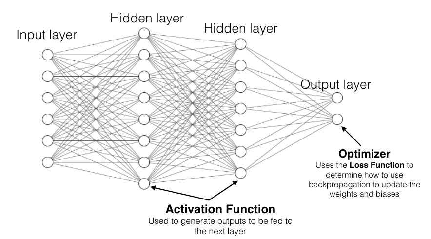
At this juncture, it's useful to refer to Figure 21, which shows how the activation function, loss function, and the optimizer work to train the neural network.
Batch Size and Epoch
In deep learning, the batch size is the number of samples processed before the weights and biases in the neural network are updated. In the example shown in the previous section, the batch size is 1. If the batch size is 5, this means the weights and biases will only be updated after sampling five rows. The weights will be updated at the end of the fifth row, based on the average of the five gradients obtained in each iteration. For example, for the first weight, you take the average of dL/dw1 obtained for each row. Then, using this average, you update the weight according to the formula described earlier.
A dataset can be divided into one or more batches. The following learning algorithms are named according to the size of each batch:
- Batch gradient descent: Batch size is the same as the size of the dataset
- Stochastic gradient descent: Batch size is 1 (i.e., the weights and biases are updated at the end of each row)
- Mini-batch gradient descent: The batch size is more than 1 and less than the size of the dataset. Popular sizes are 32, 64, and 128.
Smaller batch size requires less memory, because you're training the network using fewer samples at any one time. In addition, it's been found that a smaller batch size produces a more accurate model compared to larger batch size. Using a larger batch size can be faster compared to a smaller batch size.
The number of epochs determines how many times the learning algorithm walks through all the rows in the entire dataset. An epoch comprises of one or more batches. In real life, you often have to run your training over a large number of epochs in order for the errors to be sufficiently minimized. It's not uncommon to see epochs of 500, 1000, or more.
Finally, let's see an example to fully understand the relationships between batch size and epochs. Suppose you have a dataset of 10,000 rows. Given a batch size of 5, there will be a total of 10,000/5, or 2000 batches. This means that the weights and biases will be updated 2000 times in a single epoch. With 1000 epochs, the weights and biases will be updated a total of 2000 x 1000, or 2 million times.
TensorFlow, Keras, and Deep Learning
Developers who want to get started with deep learning can make use of TensorFlow, an open source library by Google that helps you create and train deep learning neural networks. TensorFlow has a steep learning curve and may not be easy to work with if you just want to get started with deep learning. To make TensorFlow more accessible, a Google AI researcher named Francois Chollet created Keras, an open-source neural-network library written in Python. Keras runs on top of TensorFlow and makes creating your deep learning model much easier and faster.
Using Keras to Recognize Handwritten Digits
With the theory out of the way, it's now time to look at some code and work on building your first deep neural network. For this, you'll need to install Anaconda. You'll make use of Jupyter Notebook.
Installing TensorFlow and Keras
The first step after launching Jupyter Notebook is to install TensorFlow and Keras. In the first cell of Jupyter Notebook, type the following statement:
!pip install tensorflow
The above statement installs TensorFlow and Keras on your computer.
Import the Libraries
Next, import all of the libraries that you're going to need, including NumPy, matplotlib (for charting), as well as the various classes in Keras:
import numpy as np
import matplotlib.pyplot as plt

from tensorflow.keras.datasets import mnist
from tensorflow.keras.models import Sequential
from tensorflow.keras.layers import Dense, Activation
from tensorflow.keras.optimizers import SGD
from tensorflow.keras.utils import to_categorical
from tensorflow.keras.models import Sequential
Getting the Dataset
For this example, you're going to use the MNIST (Modified National Institute of Standards and Technology) dataset, which is a large database of handwritten digits that's commonly used for training various image processing systems. The following statements loads the MNIST dataset and prints out the shape of the training and testing dataset:
(X_train, y_train), (X_test, y_test) = mnist.load_data()

print(X_train.shape)    # (60000, 28, 28)
print(y_train.shape)    # (60000,)
print(X_test.shape)     # (10000, 28, 28)
print(y_test.shape)     # (10000,)
As you can see, there are 60,000 records for the training set and 10,000 records for the testing dataset. Each handwritten digit is stored as a 28x28 two-dimensional array. If you want to see how the digits are stored, you can try printing out the first one, like this:
print(X_train[0])
You'll see a two-dimensional array containing a series of values from 0 to 255. To see what digit is represented by this array, print out its label:
print(y_train[0]) # 5
Visualizing the Dataset
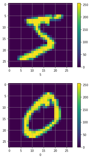
A better way to visualize the dataset is to plot it out using matplotlib. The following statements print out the first two digits in the training dataset (see Figure 22 for the output):
# show the first 2 images in the training set
for i in range(2):
    plt.figure()
    plt.imshow(X_train[i])
    plt.colorbar()
    plt.grid(True)
    plt.xlabel(y_train[i])
    plt.show()
Reshaping the Data
For training your neural network, you need to reshape (flatten) the 28x28 two-dimensional array into a single dimension. The following statements accomplish that:
NEW_SHAPE = 784              # 28x28

X_train = X_train.reshape(60000, NEW_SHAPE)
X_train = X_train.astype('float32')
print(X_train.shape)         # (60000, 784)

X_test = X_test.reshape(10000, NEW_SHAPE)
X_test = X_test.astype('float32')
print(X_test.shape)          # (10000, 784)
X_train was initially 60,000 rows of 28x28 values, but after reshaping, it will now be 60,000 x 784. Likewise for x_test after reshaping, it will be 10,000 x 784.
Normalizing the Data
You also need to convert the values of the images from a range of 0 to 255 to a new range of 0 to 1. The following statements do just that:
X_train /= 255
X_test /= 255
One-Hot Encoding
For the label of the dataset, you need to perform one-hot encoding. Essentially, one-hot encoding translates the value of the label into an array of 1s and 0s, with a single 1 representing the value and the rest filled with 0s. The best way to understand one-hot encoding is an example, such as the value 5 one-hot encoded as:
[0,0,0,0,0,1,0,0,0,0]
The value 8 is represented as:
[0,0,0,0,0,0,0,0,1,0]
Make sense now? The following statements performs a one-hot encoding for the labels stored in Y_train and Y_test:
CLASSES = 10   # number of outputs = number of digits

# convert class vectors to binary class
# matrices - one-hot encoding
Y_train = to_categorical(y_train, CLASSES)
Y_test = to_categorical(y_test, CLASSES)

# label for first row in training set
print(y_train[0])  # 5

# label (one-hot encoded) for first row in training set
print(Y_train[0])
# [0. 0. 0. 0. 0. 1. 0. 0. 0. 0.]

# second row label
print(y_train[1])
# 0

print(Y_train[1])
# [1. 0. 0. 0. 0. 0. 0. 0. 0. 0.]
Building the Model
With the dataset reshaped and encoded, you're now ready to build the neural network. Figure 23 shows the neural network that you'll build.
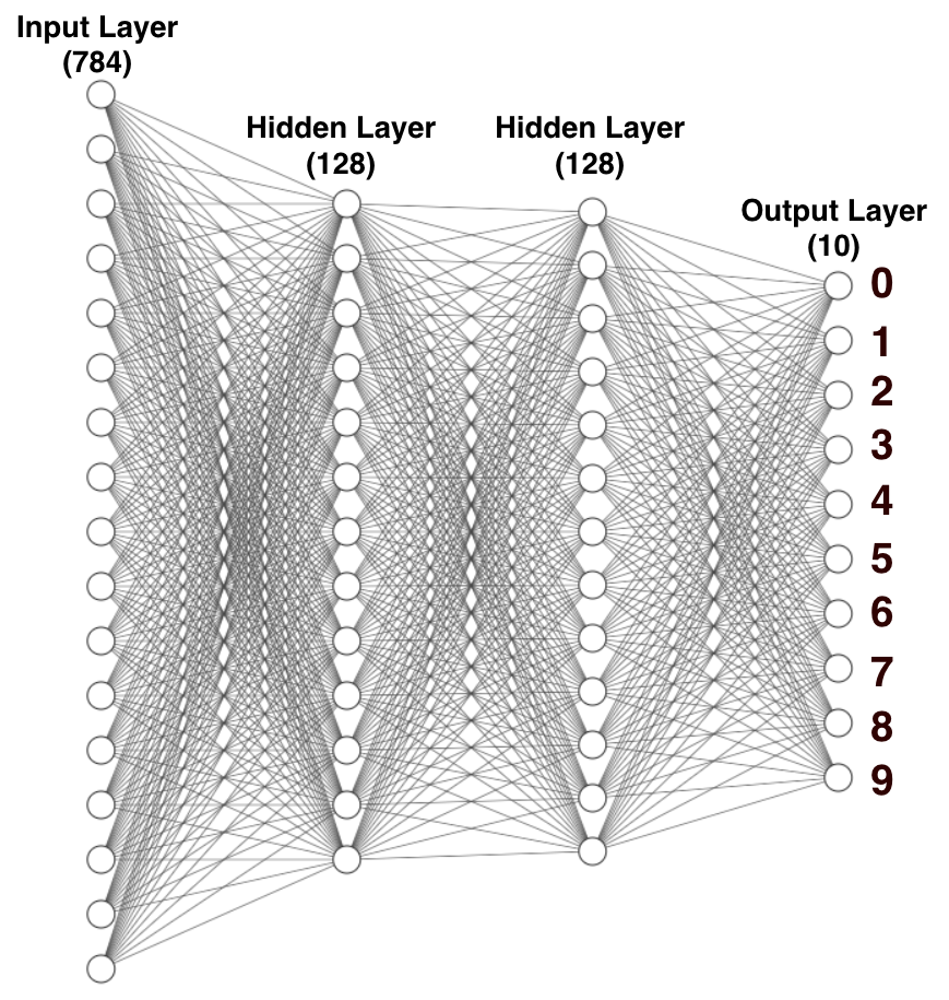
From the figure, observe that:
- There's an input layer of 784 nodes. This corresponds to the 28x28 pixels of each image. Each of the images is flattened, so each image corresponds to 784 pixels (28x28).
- Each of the 128 nodes in the first hidden layer takes in 784 inputs from the input layer and then calculates 128 outputs, which are then passed to the next hidden layer.
- Each of the 128 nodes in the second hidden layer receives the 128 inputs from the previous hidden layer and calculates 10 outputs, which are then passed to the last layer (the output layer).
- Calculated using the Softmax activation function, each neuron in the output layer contains a probability that corresponds to the digit that is currently trained/predicted.
With the model designed, it's now time to code it using Keras. Listing 1 shows the model written using Keras.
Listing 1. Building the neural network using Keras
model = Sequential()

# hidden layer 1; takes in input arrays of
# shape (*,784) and output arrays of shape (*, 128)
model.add(Dense(128, input_shape=(NEW_SHAPE,)))
# uses the ReLu activation function
model.add(Activation('relu'))

# hidden layer 2; no need to specify input (it takes
# from the previous layer); takes in input arrays of
# shape (*,128) and output arrays of shape (*, 128);
# uses ReLu
model.add(Dense(128, activation='relu'))

# output layer; takes in (*,128) and outputs (*,10)
model.add(Dense(CLASSES))
model.add(Activation('softmax'))

'''
The above 2 lines can also be written as
model.add(Dense(CLASSES, activation='softmax'))
'''
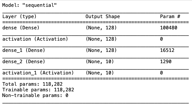
With the model created in code, it's always useful to print out the model and verify its correctness. You can do this using the summary() method of the model object:
model.summary()
You'll see the various layers of your model, as shown in Figure 24. Notice that, in this case, you have three activation functions: one each after the two hidden layers where you use the ReLU activation function, and the third one is at the output layer, where you use the softmax function to provide the probability of predicting each digit.
Compiling the Model
With the model created, you next need to compile it by specifying the loss function you want to use for this model and the optimizer you want to use for backpropagation:
model.compile(
    loss='categorical_crossentropy',
    optimizer=SGD(),
    metrics=['accuracy'])
For the example, I used the categorical cross entropy as the loss function, and the Stochastic Gradient Descent (SGD) as the optimizer for backpropagation. For the metric to measure the effectiveness of our model, I used accuracy as the metric.
Training the Model
You're now ready to train the model:
EPOCH            = 100
BATCH_SIZE       = 64
VERBOSE          = 1
VALIDATION_SPLIT = 0.2
history = model.fit(
    X_train, Y_train,
    batch_size=BATCH_SIZE,
    epochs=EPOCH,
    verbose=VERBOSE,
    validation_split=VALIDATION_SPLIT)
You specify a batch size of 64 and a validation split of 0.2 (20%). This means that when training the model with the specified dataset, 80% of the training dataset will be used for testing, while the rest (20%) will be used to verify the accuracy of the model. The fit() function returns a History object. The object stores a record of training loss values and metric values at successive epochs, as well as validation loss values and validation metrics values.
As the model trains, you'll see the output, as shown in Figure 25.
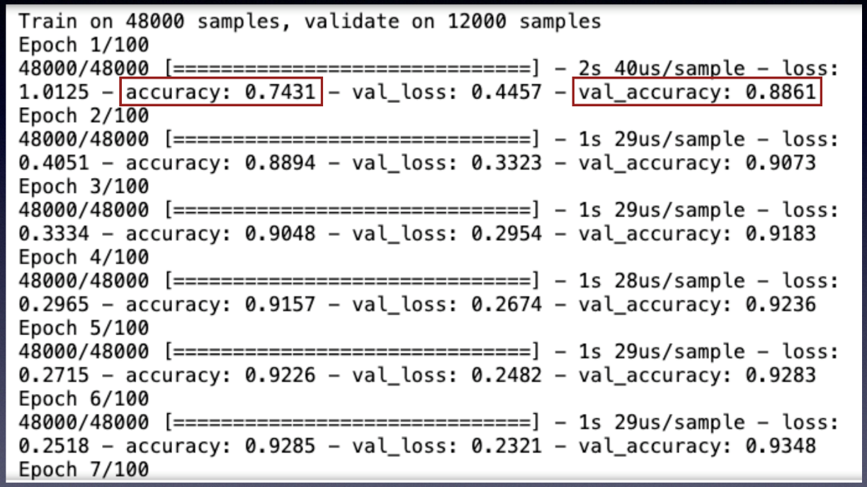
As the training goes through each epoch, it prints the training accuracy and the validation accuracy (as well as the training and validation loss). Training accuracy is obtained by applying the model on the training data.
At the early stage of training, the training accuracy should fall below the validation accuracy. After a number of epochs, the training accuracy will start to rise above the validation accuracy. This means that your model is fitting the training set better, but losing its ability to predict new data, which means that your model is starting to overfit. At this point, it's useful to stop the training.
Evaluating the Model
Once the training is done, you can evaluate the model by passing in the testing dataset to the trained model:
score = model.evaluate(X_test, Y_test, verbose=VERBOSE)
print("\nTest score:", score[0])
print('Test accuracy:', score[1])
A bunch of text will be displayed, but at the end of the output, you'll see the most important information:
Test score: 0.08266904325991636
Test accuracy: 0.9756
An accuracy of 97.56 certainly looks good!
Plotting the Training Accuracy and Validation Accuracy Chart
Using the History object returned by the fit() function, let's now plot a chart to show the training and validation accuracies of the model during the training phase:
# list all data in history
print(history.history.keys())
plt.plot(history.history['accuracy'])
plt.plot(history.history['val_accuracy'])
plt.title('model accuracy')
plt.ylabel('accuracy')
plt.xlabel('epoch')
plt.legend(['train', 'val'], loc='upper left')
plt.show()
Figure 26 shows the chart plotted.
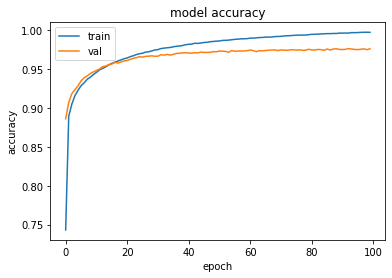
As you can see, the training accuracy out-performs validation accuracy at around 17 or 18 epochs. The ideal epoch would be around 17 or 18.
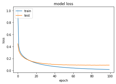
Plotting the Training Loss and Validation Loss Chart
You can also plot a chart showing the training loss and validation loss during the training phase (see Figure 27 for the chart):
plt.plot(history.history['loss'])
plt.plot(history.history['val_loss'])
plt.title('model loss')
plt.ylabel('loss')
plt.xlabel('epoch')
plt.legend(['train', 'test'], loc='upper left')
plt.show()
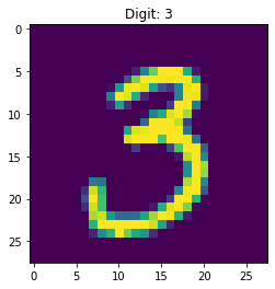
Performing Predictions
Finally, you can now make some predictions using the model that you've trained. To do so, let's select a particular row from the X_test dataset (say, index 90). In order to perform the prediction, you need to reshape the test item into an array of shapes (1,784). It's also useful to visually inspect the test row before performing the prediction:
index = 90

# shape of X_test
print(X_test.shape)                  # (10000, 784)

# shape of the first item in X_test
print(X_test[index].shape)# (784,)

# in order to do prediction, you need to send in a 2-d array of shape (,784)
x = X_test[index].reshape(-1,784)
print(x.shape)                       # (1,784)
# show the number
plt.imshow(X_test[index].reshape(28,28), interpolation='none')
plt.title("Digit: {}".format(y_test[index]))
Figure 28 shows the digit to be predicted as well as its real value.
You can now perform the prediction using the predict() function:
# you can do the prediction now
print(model.predict(x))
The above statement yields the following result:
[[7.0899937e-08 8.5124242e-08 1.1331436e-08
  9.9979192e-01 1.9511590e-13 2.1899252e-06
  4.0693807e-13 3.2966765e-11 1.3524551e-04
  7.0466805e-05]]
The first element in the result array shows the probability of the test digit being 0, and the second element shows the probability of the test digit being 1, and so on. You can observe that the fourth element (index 3) has the largest probability among all the other probabilities. Thus the predicted number is 3 (remember the digit starts from 0).
An easier way to know the predicted digit (class) is to use the predict_classes() function, which directly returns the digit predicted:
print(model.predict_classes(x)) # [3]
You can compare the result with the original one-hot encoded value of the row:
# see the original value
print(Y_test[index])
# [0. 0. 0. 1. 0. 0. 0. 0. 0. 0.]
Saving the Trained Model
Once your model is trained, you can save it to disk so that the next time you want to make a prediction, you don't have to go through the entire training process again. Although this current example doesn't take long to train, in real life, there are models that will take days, if not weeks, to train. Therefore, it's important to be able to save the trained model to disk for use later on. The following statements save the trained model as a HDF5 file:
# creates a HDF5 file 'trained_model.h5'
model.save('trained_model.h5')
Loading the Saved Model
Once the model is saved, you want to verify that it's saved properly by loading it back from disk. The following statements load the saved model:
from tensorflow.keras.models import load_model

# returns a compiled model identical to the previous one
model = load_model('trained_model.h5')
Perform a prediction using the same row that you tested earlier and you should see the same result:
print(model.predict_classes(x)) # [3]
Converting to TensorFlow Lite
Although TensorFlow allow you to train deep learning neural networks as well as make inferences (predictions) on your computer, it's useful to be able to make inferences on the edge. This is the use of TensorFlow Lite. TensorFlow Lite is a light-weight version of TensorFlow, designed specifically for inferencing on mobile devices.
For the model that you've trained, you can convert it into TensorFlow Lite using the TFLiteConverter class, as shown in the statements in Listing 2.
Listing 2. Converting the TensorFlow Model to TensorFlow Lite
# tensorflow 1.x
import tensorflow.compat.v1 as tf

# load the trained model
converter = tf.lite.TFLiteConverter.from_keras_model_file('trained_model.h5')

# convert it to tensorflow litet
flite_model = converter.convert()

# write the tensorflow lite model to disk
open("trained_model.tflite", "wb").write(tflite_model)
Saving the model as TensorFlow Lite allows your model to be used in mobile applications, such as iOS and Android apps. After the conversion is done, you'll see a number displayed, like this:
474736
This is the size of the TensorFlow Lite model saved on disk, in bytes. So the generated TensorFlow Lite model is about 475 kilobytes.
Using TensorFlow on Mobile Apps: TensorFlow Lite
Now that you're able to save your model in TensorFlow Lite, let's do something interesting. Instead of using the test dataset for verifying your model, you're going to handwrite your own digits and let the model perform the prediction on a mobile app. For this, you're going to use Flutter so that you can create the application that can run on both Android and iOS devices.
Creating the Project
I'm going to assume that you have installed Flutter on your computer. If not, check out my earlier Flutter article in CODE Magazine (https://www.codemag.com/Article/1909091/Cross-Platform-Mobile-Development-Using-Flutter).
To create a new application using Flutter, type the following commands in Terminal:
$ flutter create recognizer
$ cd recognizer
Capturing the User's Handwriting
To allow users to handwrite the digit, use a Flutter package called flutter_signature_pad. This package allows users to sign with the finger and export the result as an image.
Add the following statements in bold to the pubspec.yaml file:
dependencies:
  flutter:
    sdk: flutter
  flutter_signature_pad: ^2.0.0+1
  image:
Add the statements shown in bold in Listing 3 to the main.dart file in the lib folder of your Flutter project.
Listing 3. The statements in bold allow you to draw on your mobile app using your finger
import 'package:flutter/material.dart';
import 'dart:ui' as ui;
import 'package:flutter_signature_pad/flutter_signature_pad.dart';
import 'package:image/image.dart' as img;

void main() => runApp(MyApp());

class MyApp extends StatelessWidget {
    @override
    Widget build(BuildContext context) {
        return MaterialApp(
            title: 'Flutter Demo',
            theme: ThemeData(primarySwatch: Colors.blue,),
            home: MyHomePage(title: 'Flutter Demo Home Page'), );
    }
}

class MyHomePage extends StatefulWidget {
    MyHomePage({Key key, this.title}) : super(key: key);
    final String title;
    @override
    _MyHomePageState createState() => _MyHomePageState();
}

class _MyHomePageState extends State<MyHomePage> {
    // draw the signature in red, with width 15
    var color = Colors.red;
    var strokeWidth = 15.0;
    final _sign = GlobalKey<SignatureState>();
    String result = "";

    BoxDecoration myBoxDecoration() {
        return BoxDecoration(border: Border.all(), );
    }

    @override
    Widget build(BuildContext context) {
        return Scaffold(
            body: Center(
                child: Column(
                    mainAxisAlignment: MainAxisAlignment.center,
                    children: <Widget>[
                        Container(
                            margin: const EdgeInsets.all(10.0),
                            width: 200.0,
                            height: 200.0,
                            decoration: BoxDecoration(
                                border: Border.all(width: 3.0),
                                borderRadius: BorderRadius.all(Radius.circular(5.0)),
                            ),
                            child: Signature(
                                color: color,
                                key: _sign,
                                onSign: () {
                                    final sign = _sign.currentState;
                                },
                                strokeWidth: strokeWidth,
                            ),
                        ),
                        MaterialButton(
                            color: Colors.yellow,
                            child: Text("Recognize"),
                            onPressed: () async {
                                final sign = _sign.currentState;

                                // get the signature data
                                final sigImage = await sign.getData();

                                // convert to png format
                                var data = await sigImage.toByteData(format: ui.ImageByteFormat.png);
                                final buffer = data.buffer;
                                var imageBytes = buffer.asUint8List(data.offsetInBytes, data.lengthInBytes);
                                img.Image image = img.decodePng(imageBytes);

                                // resize the image
                                image = img.copyResize(image, width:28);

                                // clear signature pad
                                sign.clear();
                            },
                        ),
                        MaterialButton(
                            child: Text("Clear"),
                            color: Colors.lime,
                            onPressed: () {
                                final sign = _sign.currentState;
                                sign.clear();
                                setState(() {
                                    result = "";
                                });
                                debugPrint("cleared");
                            },
                        ),
                        Text('$result',
                            style: TextStyle(fontWeight: FontWeight.bold, fontSize: 20,
                        ),
                        textDirection: TextDirection.ltr,),
                    ]
                ),
            ),
        );
    }
}
Let's give the app a spin and see how you can scribble on the signature pad. In Terminal, type the following command to launch the app on the iPhone Simulator:
$ open -a simulator
$ flutter run -d all
You can now scribble on the signature pad and tap Clear to restart (see Figure 29).
Using TensorFlow Lite
Now that you can scribble on the app, let's use the TensorFlow Lite model to predict the digit that you've scribbled. In the project folder, add a new folder named model (see Figure 30):
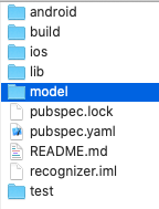
Create a plain text file named trained_model.txt with the following contents and save it to the model folder:
Zero
One
Two
Three
Four
Five
Six
Seven
Eight
Nine
This file contains the labels for the predictions. If the prediction is 0, it will look for the first line in the file and return “Zero”, and so on. Of course, you can replace “Zero” with any value you want, such as 0, or any value of your preference.
Next, add the trained_model.tflite file that you have converted earlier into the model folder.
To bundle the both the trained_model.tflite and trained_model.txt files with your Flutter app, add the following statements in bold to the pubspec.yaml file:
dependencies:
  flutter:
    sdk: flutter
  flutter_signature_pad: ^2.0.0+1
  image:
  tflite: ^1.0.4
...
...
flutter:
  assets:
   - model/trained_model.tflite
   - model/trained_model.txt
The tflite package is a Flutter plug-in for accessing TensorFlow Lite API. It supports image classification, object detection (SSD and YOLO), Pix2Pix and Deeplab, and PoseNet on both iOS and Android.
Add the statements in bold from Listing 4 to the main.dart file. Use the Tflite.runModelOnBinary() function is used for image classification (refer to https://pub.dev/documentation/tflite/latest/ for more examples).
Listing 4. Loading the TensorFlow Lite model
import 'dart:typed_data';
import 'package:flutter/services.dart';

import 'package:flutter/material.dart';
import 'dart:ui' as ui;
import 'package:flutter_signature_pad/flutter_signature_pad.dart';
import 'package:image/image.dart' as img;
import 'package:tflite/tflite.dart';

void main() => runApp(MyApp());

...
class _MyHomePageState extends State<MyHomePage> {
    var color = Colors.red;
    var strokeWidth = 15.0;
    final _sign = GlobalKey<SignatureState>();
    String result = "";

    //---load the TensorFlow Lite model---
    Future loadModel() async {
        Tflite.close();
        try {
            String res;
            res = await Tflite.loadModel(
                model: "model/trained_model.tflite",
                labels: "model/trained_model.txt");
            print(res);
        } on PlatformException {
            print('Failed to load model.');
            print(PlatformException);
        }
    }

    Future recognizeImageBinary(var imageBytes) async {
        var recognitions = await Tflite.runModelOnBinary(
            binary: imageToByteListFloat32(imageBytes, 28),
            numResults: 9,
            threshold: 0.8,
            asynch: true);
        print(recognitions);
        double highestConfidence = 0;
        String predictedDigit = "Not Recognized";
        for (final i in recognitions) {
            if (i['index'] <10 && i['confidence'] > highestConfidence) {
                predictedDigit = i['label'];
            }
        }
        setState(() {
            result = predictedDigit;
        });
    }

    Uint8List imageToByteListFloat32(img.Image image, int inputSize) {
        //  the model has an input shape of 1x28x28x1
        var convertedBytes = Float32List(1 * inputSize * inputSize * 1);
        var buffer = Float32List.view(convertedBytes.buffer);
        int pixelIndex = 0;
        for (var i = 0; i < inputSize; i++) {
            for (var j = 0; j < inputSize; j++) {
                var pixel = image.getPixel(j, i);
                buffer[pixelIndex++] = (img.getRed(pixel)) / 255;
            }
        }
        return convertedBytes.buffer.asUint8List();
    }

    @override
    void initState() {
        super.initState();
        loadModel();
    }

    BoxDecoration myBoxDecoration() {
        return BoxDecoration(border: Border.all(), );
    }

    @override
    Widget build(BuildContext context) {
        return Scaffold(
            body: Center(
                ...
                MaterialButton(
                    color: Colors.yellow,
                    child: Text("Recognize"),
                    onPressed: () async {
                        final sign = _sign.currentState;
                        ...

                        // resize the image
                        image = img.copyResize(image, width:28);

                        // perform prediction
                        recognizeImageBinary(image);

                        // clear signature pad
                        sign.clear();
                    },
                ),
                MaterialButton(
                    ...
                ),
                Text('$result',
                    style: TextStyle(fontWeight: FontWeight.bold, fontSize: 20,),
                    textDirection: TextDirection.ltr, ),
                ),
            ),
        );
    }
}
One possible result of the Tflite.runModelOnBinary() function might look like this (formatted for clarity):
[
  {
    index: 10,
    label: Nine,
    confidence: 1.2579584121704102
  },
  {
    index: 3,
    label: Three,
    confidence: 0.6730967641398132
  },
  {
    index: 2,
    label: Two,
    confidence: 0.9919105172157288
  }
]
You need to iterate through the result and find those items whose index value is from 0 to 9 (because you're predicting digits from 0 to 9), and get the one with the highest confidence.
For iOS
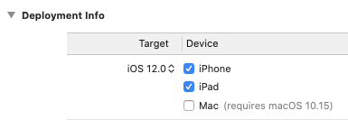
You need to modify the iOS component of the project before you can run it. In the ios folder of the project, open the Runner.xcworkspace file in Xcode.
Change the Target to iOS 12.0 (see Figure 31):
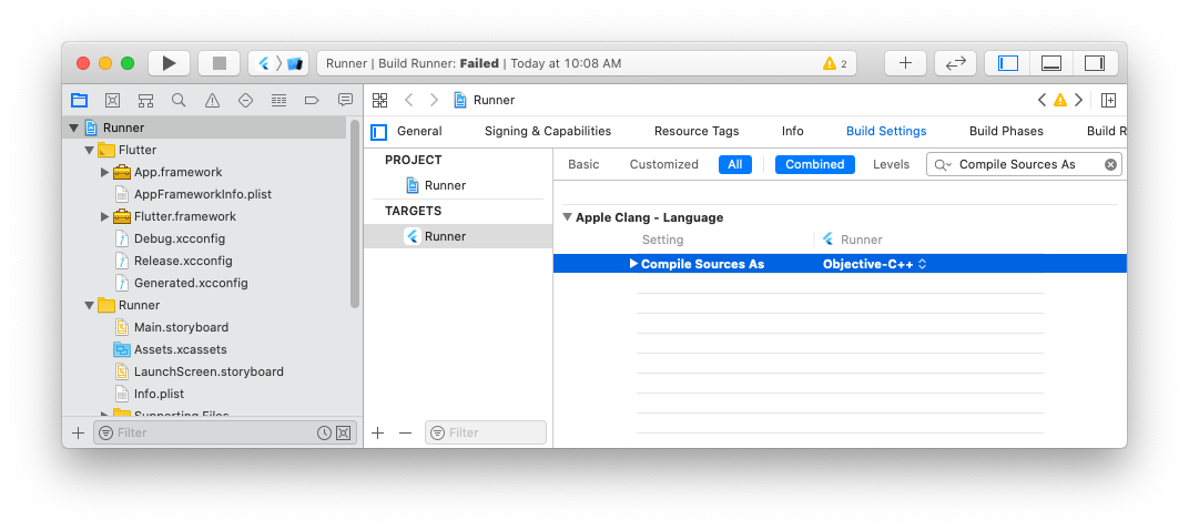
Also, go to the page Runner > Targets > Runner > Build Settings, search for Compile Sources As, and change the value to Objective-C++ (see Figure 32).
For Android
For the Android component of your Flutter app, add the statements in bold (see Listing 5) to the build.gradle file in the android/app folder.
Listing 5. Adding the statements to the build.gradle file
android {
    compileSdkVersion 28

    sourceSets {
        main.java.srcDirs += 'src/main/kotlin'
    }

    lintOptions {
        disable 'InvalidPackage'
    }

    defaultConfig {
        applicationId "com.example.recognizer"
        minSdkVersion 19
        targetSdkVersion 28
        versionCode flutterVersionCode.toInteger()
        versionName flutterVersionName
        testInstrumentationRunner "android.support.test.runner.AndroidJUnitRunner"
    }

    buildTypes {
        release {
            signingConfig signingConfigs.debug
        }
    }
    aaptOptions {
        noCompress 'tflite'
        noCompress 'lite'
    }
}
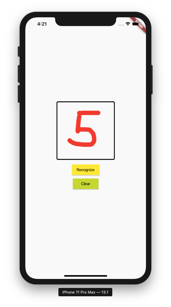
Testing the Application
That's it! You're now ready to make a prediction on the digit that you are going to scribble on your mobile app. In Terminal, type the following command:
$ flutter run -d all
If you encounter an error involving cocoapods, type the following command in Terminal:
$ sudo gem install cocoapods
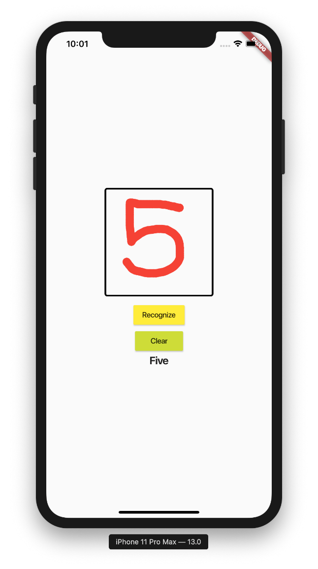
Scribble a digit and click on the Recognize button. You should now be able to use the application to recognize your handwritten text (see Figure 33).
Summary
Phew! In this article, I've covered a lot of ground on deep learning. Although there's no way a single article can discuss everything on this very complex topic, I hope I've given you a clear idea of what deep learning is and what it can do. Specifically, we have discussed:
- What deep learning is
- What activation functions are and why you need them
- What an optimizer is and how it helps to improve the performance of your neural network
- How backpropagation works
- How to build a neural network using TensorFlow and Keras
- How to train a neural network
- How to save a trained neural network to disk and export it to TensorFlow Lite so that you can perform inferencing on the edge (on a mobile device)
- How to build a Flutter application to perform handwriting recognition
Be sure to try out the examples. Have fun with deep learning!
