Developing Dashboards Using Grafana

In my earlier article on Building Dashboards Using Bokeh, I talked about how you can build dashboards programmatically using the Bokeh Python library. What if you want to create dashboards but don't want to spend too much time coding them? The good news is that you can do that using a tool called Grafana.

In this article, I'll walk you through how to get started with Grafana, and how you can use it to build interesting dashboards. I'll also describe two projects that you can build using Grafana:

• How to create dynamic auto-updated time series charts
• How to display real-time sensor data using MQTT

Installing Grafana

The first good news about Grafana is that it's free to use for most use cases, except where you need enterprise features such as advanced security, reporting, etc. If you want to modify the source code of Grafana, be sure to check the licensing info at https://grafana.com/licensing/.

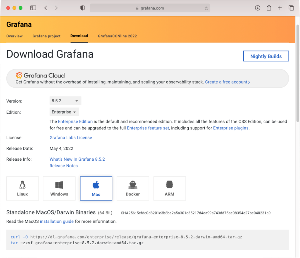
To download the free enterprise version of Grafana, go to https://grafana.com/grafana/download (see Figure 1). There, you'll find the instructions to download Grafana for the OS that you're running.

Figure 1: Instructions for downloading Grafana for the various OSes

For Windows, you can download the Windows Installer (https://dl.grafana.com/enterprise/release/grafana-enterprise-8.5.2.windows-amd64.msi) and then run it.

For Mac, you can download and install Grafana directly using Terminal:

$ curl -O https://dl.grafana.com/enterprise/release/
    grafana-enterprise-8.5.2.darwin-amd64.tar.gz

$ tar -zxvf grafana-enterprise-8.5.2.darwin-amd64.tar.gz

Once the above steps are done, you should now find a folder named Grafana-8.5.2 in your home directory. On Windows, Grafana will be installed in the following directory: C:\Program FilesGrafanaLabs\grafana\.

Starting the Grafana Service

On the Mac, you need to manually start the Grafana service by using the following commands in Terminal:

$ cd ~
$ cd grafana-8.5.2
$ ./bin/grafana-server web

On Windows, Grafana is installed as a Windows service and is automatically started after you have installed it.

Logging in to Grafana

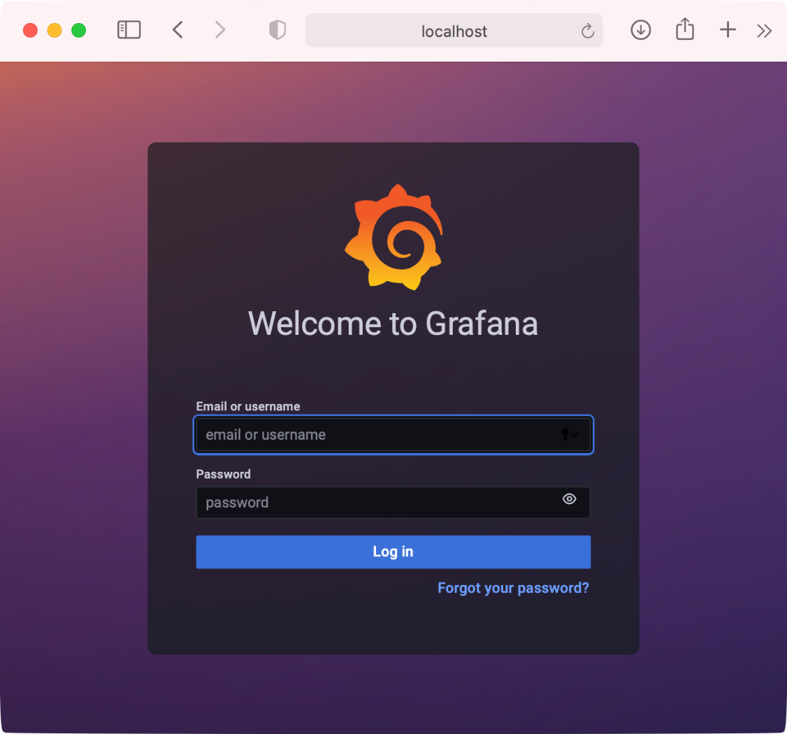
Once Grafana has been installed on your computer, open it using a Web browser using the following URL: http://localhost:3000/login (see Figure 2).

Figure 2: Logging in to Grafana

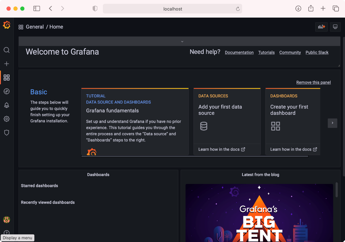
The default username is admin and password is also admin. Once you've logged in, you'll be asked to change your default password. After that, you'll see the page shown in Figure 3.

Figure 3: The home page of Grafana

If you forget your password, you can reset the admin password using the following command: ./bin/grafana-cli admin reset-admin-password password

Creating Data Sources

Grafana can load data from a variety of data sources, such as Prometheus, MySQL, InfluxDB, PostgreSQL, Microsoft SQL Server, Oracle, MongoDB, and more. If the data source that you need isn't available, you can locate additional data sources via plug-ins (Settings > Plugins). A good example of a data source that a lot of data analysts use is CSV, which is supported in Grafana through the CSV data source plug-in.

Although you can use CSV as a data source in Grafana, querying your data (and manipulating it) is much easier if you use a database data source, such as MySQL. For this article, I'll show you how to import your CSV file into a MySQL database server and then use MySQL as the data source in Grafana.

Preparing the MySQL databases

For this article, I'm going to assume that you already have MySQL and MySQL Workbench installed. In the MySQL Workbench, log in to your local database server. Create a new query and enter the following SQL statements to create a new account named user1 with password as the password:

CREATE USER 'user1'@'localhost' IDENTIFIED BY 'password';
GRANT ALL ON *.* TO 'user1'@'localhost'

Next, create a new database named Insurance:

CREATE DATABASE Insurance;
USE Insurance;

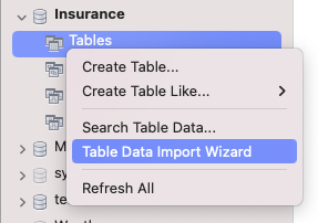
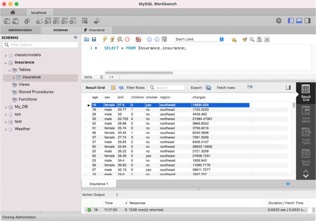
Once the Insurance database is created on MySQL, right-click on Tables and select Table Data Import Wizard (see Figure 4):

Figure 4: Import data into the table.

You'll be loading a CSV file into the Insurance database. For this example, I'll use the insurance dataset from: https://www.kaggle.com/datasets/teertha/ushealthinsurancedataset.

In the Table Data Import Wizard that appears, enter the path of the CSV file that you've downloaded and follow the steps. Specify that the data of the CSV file be loaded onto the Insurance database and you also have the option to name the table. If you take the default options, the content of the CSV file is loaded onto a table named Insurance. You should now be able to see the imported table and its content (see Figure 5).

Figure 5: Viewing the imported Insurance dataset

Using the MySQL Data Source

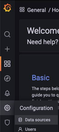
With the database prepared, it's now time to configure the MySQL data source in Grafana. In Grafana, click Configuration > Data sources (see Figure 6).

Figure 6: Configuring a new data source

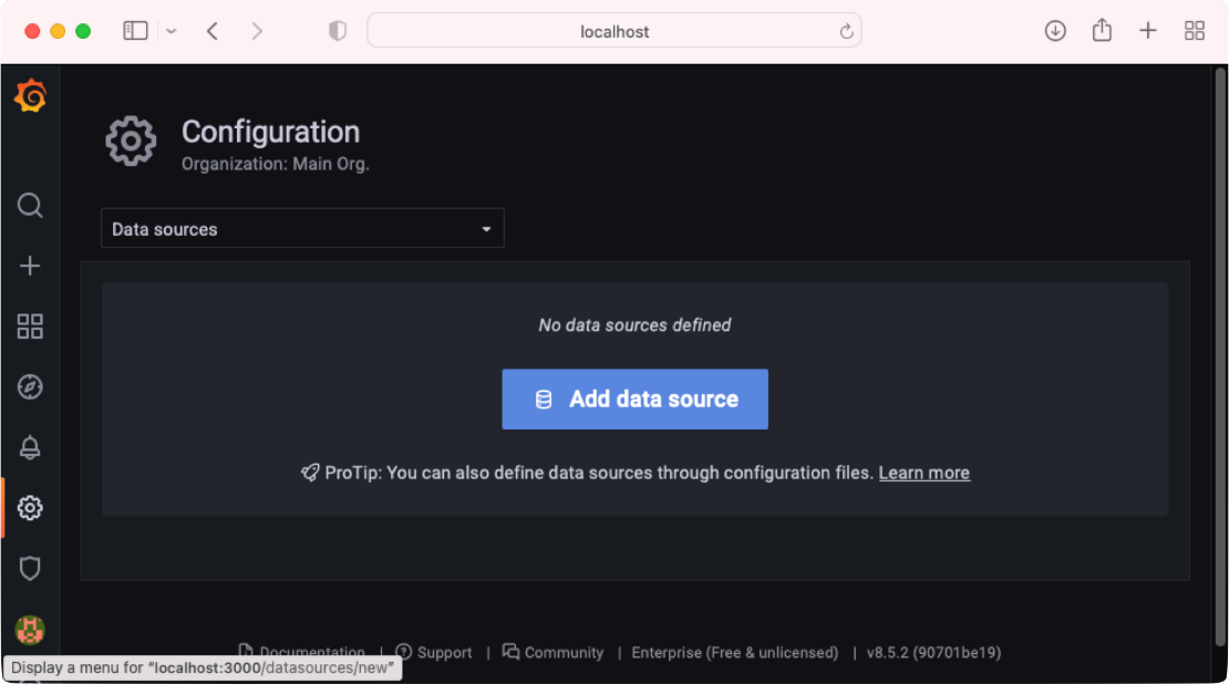
Click Add data source (see Figure 7).

Figure 7: Add a new data source.

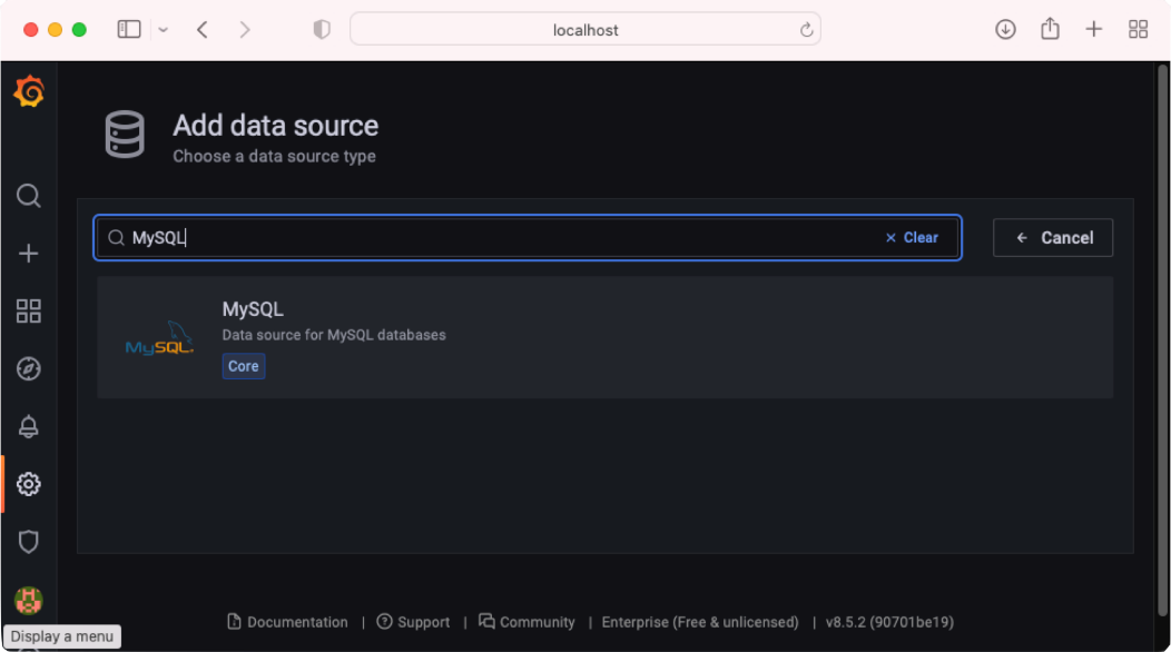
Type in MySQL and then click on the MySQL data source that appears (see Figure 8).

Figure 8: Locate the MySQL data source.

Enter the details of the MySQL connection as shown in Figure 9.

Figure 9: Configure the MySQL data source to connect to the Insurance database.

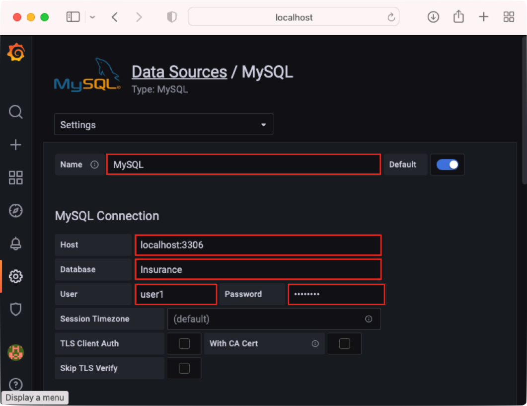
On the bottom of the page, click Save & test to ensure that the connection to the MySQL database server is working correctly.

Creating a Dashboard

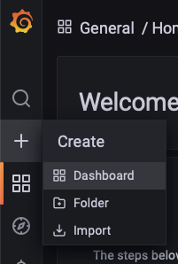
Now that the data source configuration is done, it's time to get into the meat of what we want to do! In Grafana, select + > Dashboard to create a new dashboard (see Figure 10).

Figure 10: Add a new dashboard.

In Grafana, a dashboard is a set of one or more panels organized and arranged into one or more rows.

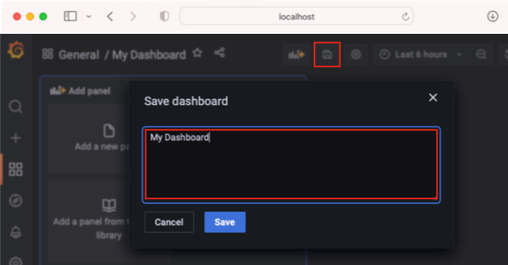
Click on the Save icon and give a name to your dashboard (see Figure 11). Click Save.

Figure 11: Name and save the dashboard.

Creating Panels

With the dashboard created, you're now ready to add a panel to your dashboard.

The panel is the basic visualization building block in Grafana. A panel can display a bar chart, pie chart, time series, map, histogram, and more.

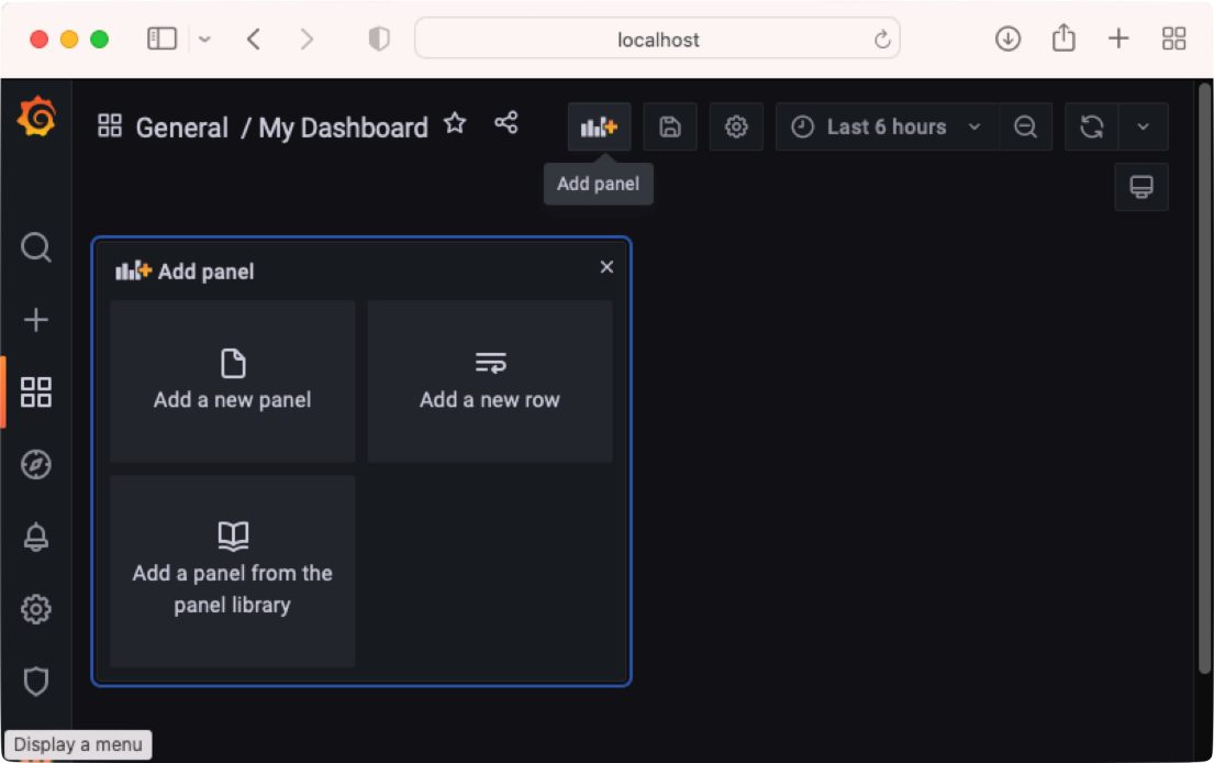
Click the Add panel icon and then the Add a new panel button to add a panel to your dashboard (see Figure 12).

Figure 12: Add a new panel to the dashboard.

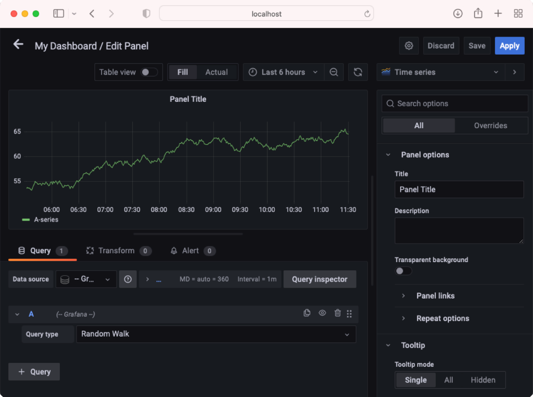
You should see the default panel, as shown in Figure 13.

Figure 13: The default panel added to the dashboard

Let's try to create a pie chart. Enter the details shown in Figure 14.

Figure 14: Display a pie chart in the current panel.

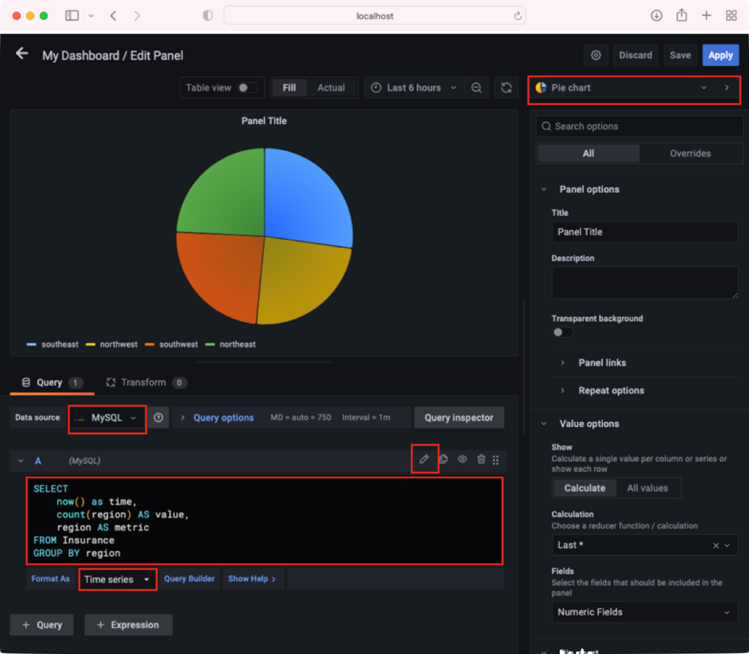
In the above, you set:

• Visualization type to Pie chart
• Data source to MySQL
• Manually set the SQL query to:

SELECT
    now() as time,
    count(region) AS value,
    region as metric
FROM Insurance
GROUP BY region

• Format to Time Series

Time series visualization is the default and primary way to visualize data in Grafana. Your SQL query's result should have a field named Time.

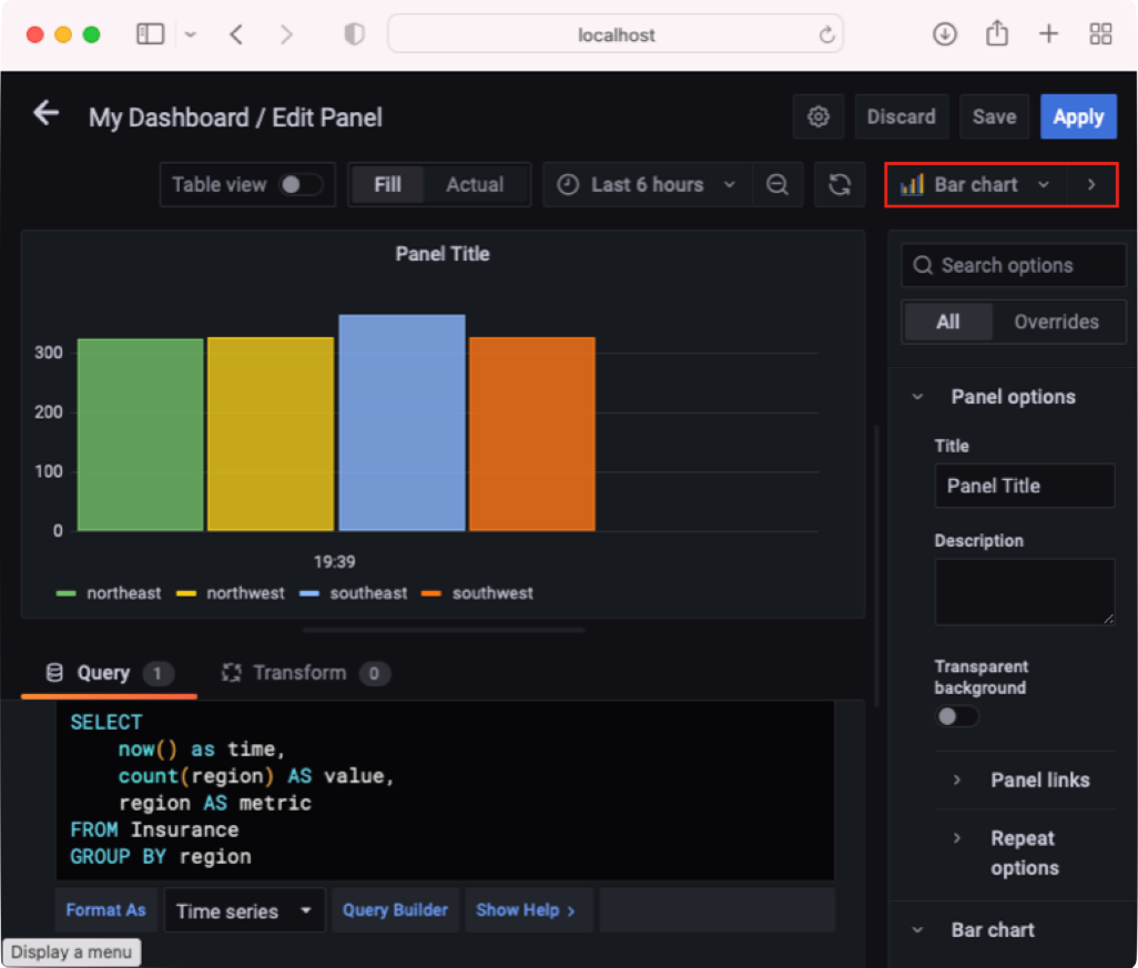
In addition to the pie chart, you can also display bar chart (see Figure 15).

Figure 15: Displaying a bar chart in the current panel

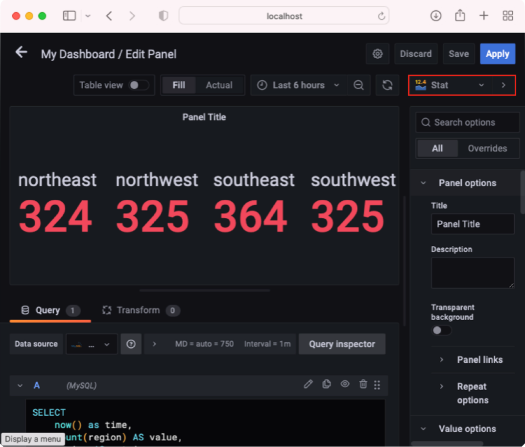
You can also display the data as Stat (statistics; see Figure 16).

Figure 16: Displaying the result of the query as statistics

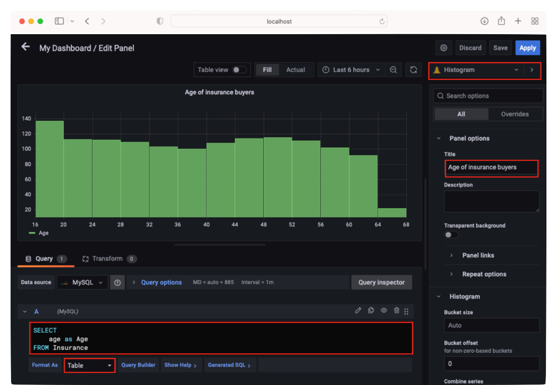
If you want to display a histogram showing the distribution of the age range, you can set the panel as shown in Figure 17.

Figure 17: Displaying a histogram showing the age distribution

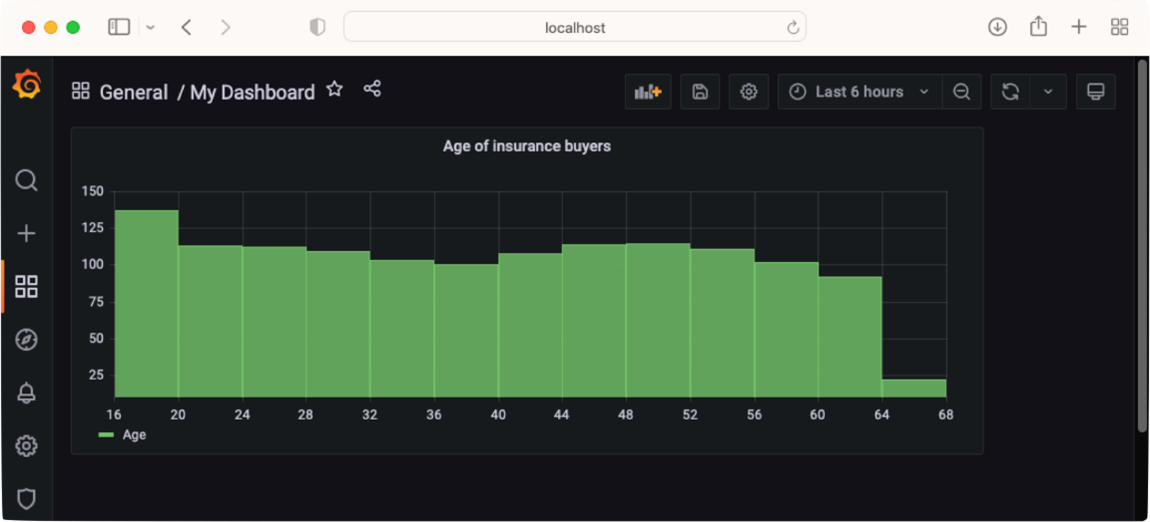
When you're done with the panel, clicking on the Apply button at the top of the page returns you to the dashboard. Your dashboard now has one panel (see Figure 18).

Figure 18: The dashboard with one panel

From this point, you can add additional panels to your dashboard.

Exporting and Importing Dashboards

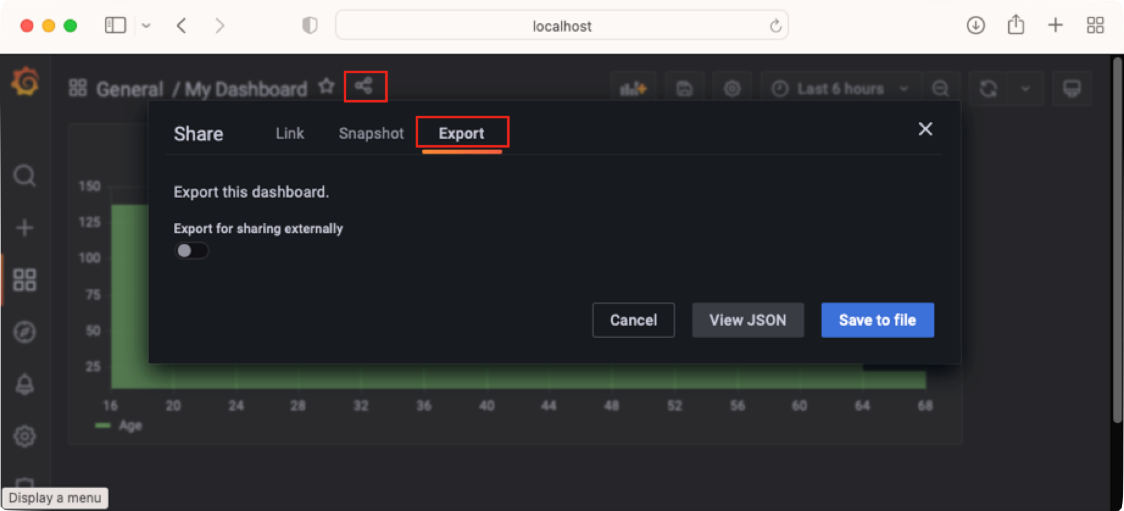
Once you've created your dashboard, you can export it so that you can back them up or load them into Grafana on another computer. To export a dashboard, click the Share icon and then click the Export tab (see Figure 19). Then, click the Save to file button.

Figure 19: Exporting a dashboard

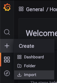
A JSON file will now be downloaded to your computer. The JSON file now contains all the details of your dashboards and can be sent to another computer. To import the exported dashboard, select + > Import (see Figure 20) and load the JSON file that you saved earlier. The dashboard will now be imported into Grafana.

Figure 20: Importing a dashboard

Creating Dynamic Auto-Updated Time Series Charts

So far in this article, you've seen how to load data from a MySQL database using the MySQL data source. However, in real-life, a lot of times the data is from Web APIs, and so it makes sense to be able to use Web APIs in Grafana. Although this looks like a straight-forward affair, it's more involved than you would imagine. For this section, you'll:

• Build a REST API back-end containing stock prices so that it can be used by Grafana's SimpleJson data source.
• Build the front-end using Grafana. The chart that you'll build shows the stock price of either AAPL or GOOG (fetched from the back-end REST API) and will be automatically updated every five seconds.

Creating the Sample Data

First, let's start off with the server side. For this project, you'll build a REST API that allows a client to retrieve the stock prices of either AAPL or GOOG based on a specified range of dates. For the stock prices, I'm going to simulate the prices by randomly generating them and then saving them in CSV files.

In the real-world, your stock data will more likely come from databases that are updated dynamically.

For this article, I'll pre-generate the prices for four days, from one day before the current day, to three days after the current day. First, generate the simulated stock prices for GOOG:

from datetime import timedelta, timezone
import datetime
import numpy as np
import pandas as pddate_today = \datetime.datetime.now()

days = pd.date_range(date_today - timedelta(1),
  date_today + timedelta(3), freq = '5s', tz = timezone.utc)

df = pd.DataFrame(
    {
        'value':np.random.uniform(2500,3200,len(days))
    }, index = days)

display(df)
df.to_csv('stocks_goog.csv')

The simulated stock price is saved as stocks_goog.csv. Next, generate the prices for AAPL:

from datetime import timedelta, timezone
import datetime
import numpy as np
import pandas as pddate_today = \datetime.datetime.now()

days = pd.date_range(date_today - timedelta(1),
  date_today + timedelta(3), freq = '5s', tz = timezone.utc)

df = pd.DataFrame(
    {
        'value':np.random.uniform(150,190,len(days))
    }, index = days)

display(df)
df.to_csv('stocks_aapl.csv')

The simulated stock price is saved as stocks_aapl.csv. Here is a sample output for the stocks_aapl.csv file:

,value
2022-03-16 11:19:56.209523+00:00,184.55338767944096
2022-03-16 11:20:01.209523+00:00,168.76885410294773
2022-03-16 11:20:06.209523+00:00,188.02816186918278
2022-03-16 11:20:11.209523+00:00,164.63482117646518
2022-03-16 11:20:16.209523+00:00,161.33806737466773
2022-03-16 11:20:21.209523+00:00,169.10779687119663
2022-03-16 11:20:26.209523+00:00,169.90405158220707
2022-03-16 11:20:31.209523+00:00,189.30501099950166
...

Creating the REST API

Let's now focus attention on creating the REST API, which is the more challenging aspect of this project. As mentioned earlier, you can use the SimpleJson data source on Grafana to connect to a REST API. However, it requires the REST API to implement specific URLs (see https://grafana.com/grafana/plugins/grafana-simple-json-datasource/ for more details). This means that your REST API must be written specially for the SimpleJson data source.

To make my life simpler, I decided to use the Grafana pandas datasource module (https://github.com/panodata/grafana-pandas-datasource) to create my REST API. This module runs an HTTP API based on Flask, and it returns Panda's dataframes to Grafana, which is what SimpleJson data source can work with. This module also provides samples where you can see how you can implement your own REST API. I've adapted one of the provided samples (sinewave-midnights) and modified it for my purposes.

Create a new text file and name it demo.py. Populate it with the following statements, shown in Listing 1.

Listing 1: The REST API for stock prices

import numpy as np
import pandas as pd
from grafana_pandas_datasource import create_app
from grafana_pandas_datasource.registry import data_generators as dg
from grafana_pandas_datasource.service import pandas_component

from datetime import datetime, timedelta
from pytz import timezone

def define_and_register_data():
    def get_stock(stock_symbol, ts_range):
        if stock_symbol == 'AAPL':
            df = pd.read_csv('stocks_aapl.csv',
                parse_dates=True, index_col=0)
        if stock_symbol == 'GOOG':
            df = pd.read_csv('stocks_goog.csv',
                parse_dates=True, index_col=0)

        # return the rows that falls within the specified dates
        return df[(df.index > ts_range['$gt']) &
            (df.index < ts_range['$lte'])]

        # Register data generators
        dg.add_metric_reader("symbol", get_stock)

def main():
    # Define and register data generators.
      define_and_register_data()

    # Create Flask application.app = create_app()

    # Register pandas component.
      app.register_blueprint(pandas_component, url_prefix="/")

    # Invoke Flask application.
      app.run(host="127.0.0.1", port=3003, debug=True)

if __name__ == "__main__":main()

Observe the following:

• The define_and_register_data() function contains another function called get_stock().
• The add_metric_reader() function links the query sent by Grafana with the function that handles the query. In this case, it will link the "symbol" query with the get_stock() function.
• The query sent by Grafana includes a value. For example, you can configure Grafana to send a query “symbol:AAPL”. The value of “AAPL” will be passed to the first parameter of the get_stock() function (see Figure 21).

Figure 21: Understanding how the REST API works with Grafana

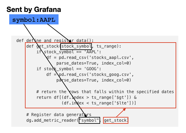
• The second parameter of the get_stock() function - a ts_range - gets its value from Grafana. You'll see this later.
• In the get_stock() function, you load the required CSV file and then perform a filter to only return the rows that match the time range (ts_range) passed in by Grafana. In real-life, you should load the data from a database server.
• The REST API listens at port 3003 on the local computer.

Before you can run the REST API, you need to install the grafana-pandas-datasource module:

$ pip install grafana-pandas-datasource

You now can run the REST API:

$ python demo.py

You should see the following:

* Serving Flask app "grafana_pandas_datasource"
(lazy loading)

* Environment: production
WARNING: This is a development server. Do not use
it in a production deployment. Use a production
WSGI server instead.

* Debug mode: on
2022-03-17 13:37:38,454.454 [werkzeug]

INFO:  * Running on http://127.0.0.1:3003/
(Press CTRL+C to quit)
2022-03-17 13:37:38,455.455 [werkzeug]

INFO:  * Restarting with stat
2022-03-17 13:37:38,895.895 [werkzeug]

WARNING:  * Debugger is active!
2022-03-17 13:37:38,902.902 [werkzeug]

INFO:  * Debugger PIN: 301-215-354

Testing the REST API

You can now test the REST API. You can issue the following command using the curl utility:

$curl -H "Content-Type: application/json" -X POST
  http://127.0.0.1:3003/query -d '{"targets":
  [{"target": "symbol:GOOG"}], "range": {"from":
  "2022-03-17 03:00:49.110000+00:00",
  "to": "2022-03-17 03:05:49.110000+00:00"}}'

The result looks like this:

[
    {
        "datapoints": [
            [3169.441653300435, 1647486052594],
            [2748.501265212758, 1647486057594],
            [3195.3559754568632, 1647486062594],
            ...
            [2744.0582066482057, 1647486342594],
            [3098.521949302881, 1647486347594]
        ],
        "target": "value"
    }
]

Each value in the datapoint array contains the stock price, as well as the epoch time. You can use the Epoch time converter at https://www.epochconverter.com to convert the value of 1647486052594, which yields the date of Thursday, 17 March 2022 03:00:52.594 (GMT).

Now that the REST API is up and running, the next thing is to work on the Grafana side.

Adding the SimpleJson data source

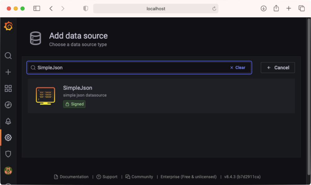
The next step is to add and configure the SimpleJSON data source in Grafana. Using the SimpleJSON data source, you can connect to REST APIs and download the data in JSON format.

In Grafana, first add a new data source (Configuration > Data sources). Click on the Add data source button. Search for SimpleJson and double click on it (see Figure 22).

Figure 22: Add the SimpleJson data source to the project.

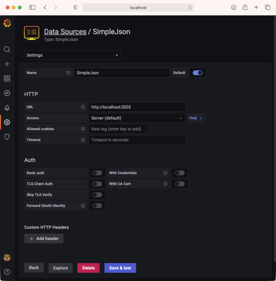
For the URL, enter http://localhost:3003 and click Save & test (see Figure 23).

Figure 23: Configure the SimpleJson data source.

Creating the Dashboard

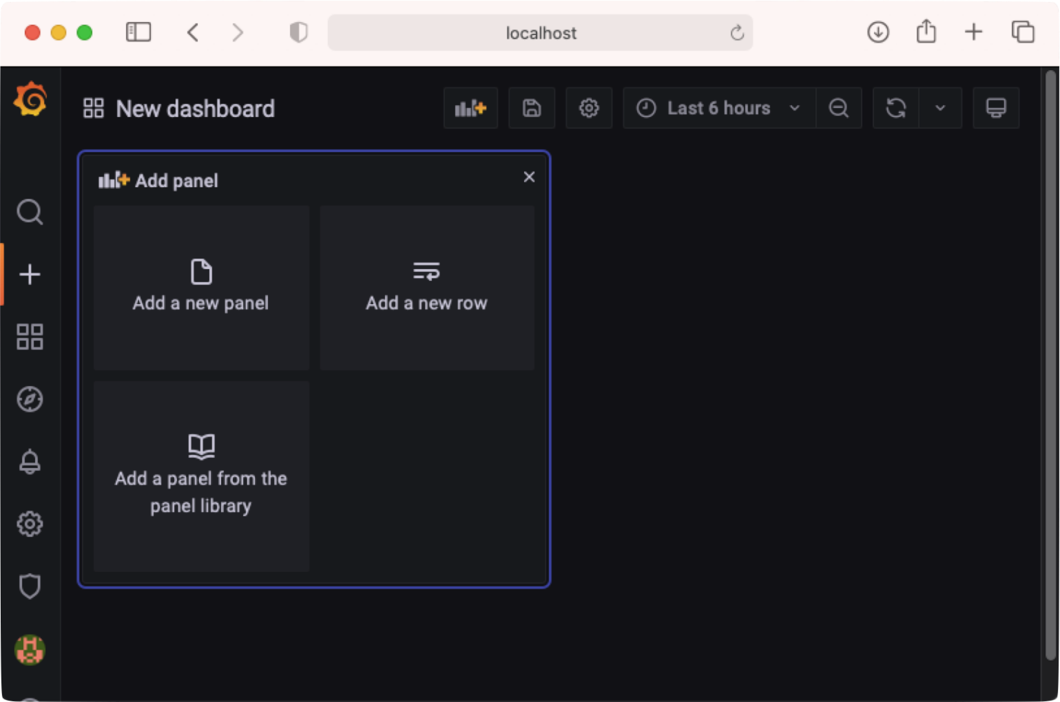
Create a new dashboard in Grafana. Then add a new panel by clicking Add a new panel (see Figure 24).

Figure 24: Add a new panel to the dashboard.

Using the default Time series visualization, configure the Data source as shown in Figure 25. Also, enter symbol:AAPL for the timeserie query. You should now see the chart plotted.

Figure 25: Configure the SimpleJson data source in the panel.

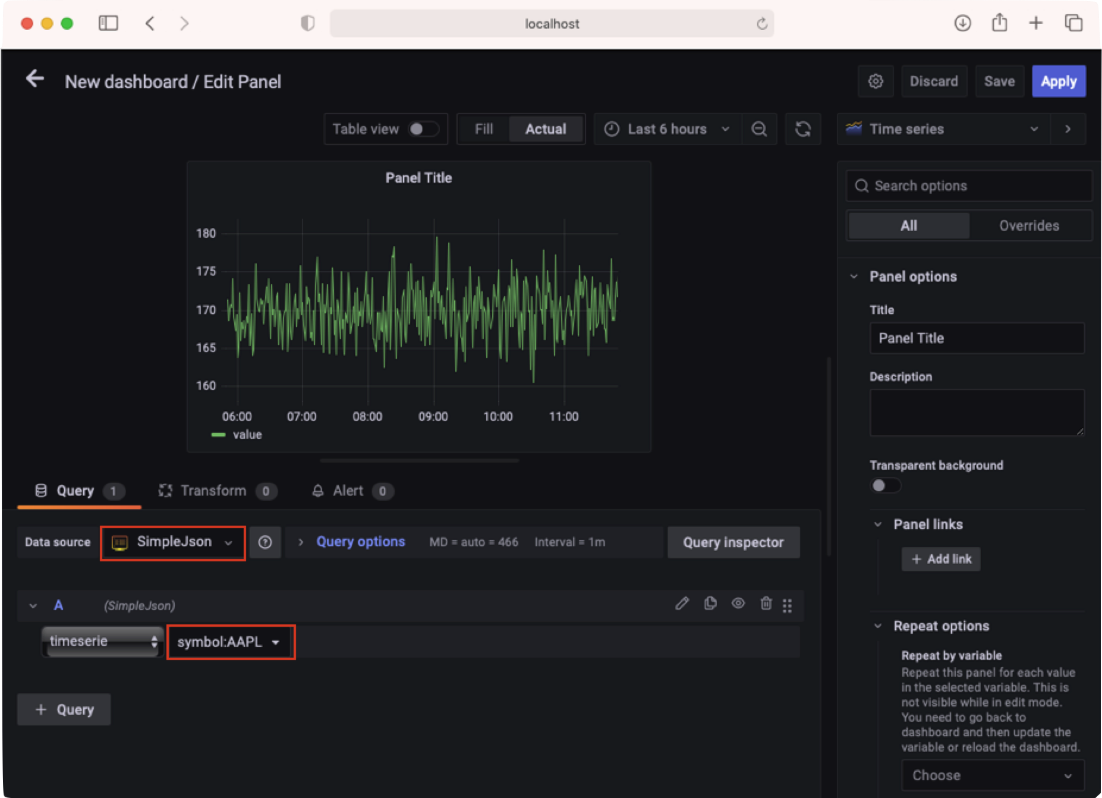
Earlier I mentioned that Grafana will send a query to the REST API. This is the query: symbol:AAPL.

You can control how often you want Grafana to fetch the data for you by selecting the date range (see Figure 26).

Figure 26: Select how often you want Grafana to fetch your data for you.

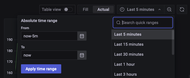
For example, if the current date and time is 17th March 2022, 5.53am (UTC-time), Grafana will send the following time range to the back-end REST API if you select the Last 5 minutes option:

{
  '$gt': datetime.datetime(2022, 3, 17, 5, 48, 18, 555000,
                           tzinfo=<UTC>),
  '$lte': datetime.datetime(2022, 3, 17, 5, 53, 18, 555000,
                            tzinfo=<UTC>)
}

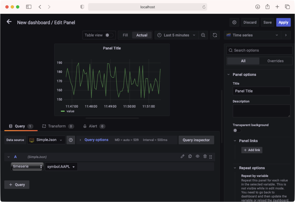
The chart will be updated with the data for the last five minutes (see Figure 27).

Figure 27: Display the data fetched from the REST API.

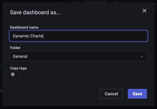
Click the Save button at the top right corner to name and save the dashboard (see Figure 28).

Figure 28: Save the dashboard.

You'll now be returned to the dashboard.

Configuring a Variable

You can configure a variable in Grafana for your dashboard to allow users to display the chart for different stock symbols.

In Grafana, a variable is a placeholder for a value that you can reference in your queries and panels.

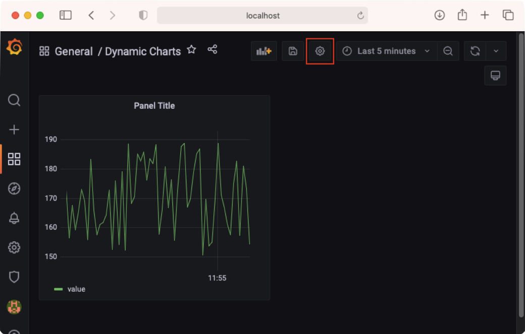
Click on the Settings button for your current dashboard (see Figure 29).

Figure 29: Configure the dashboard

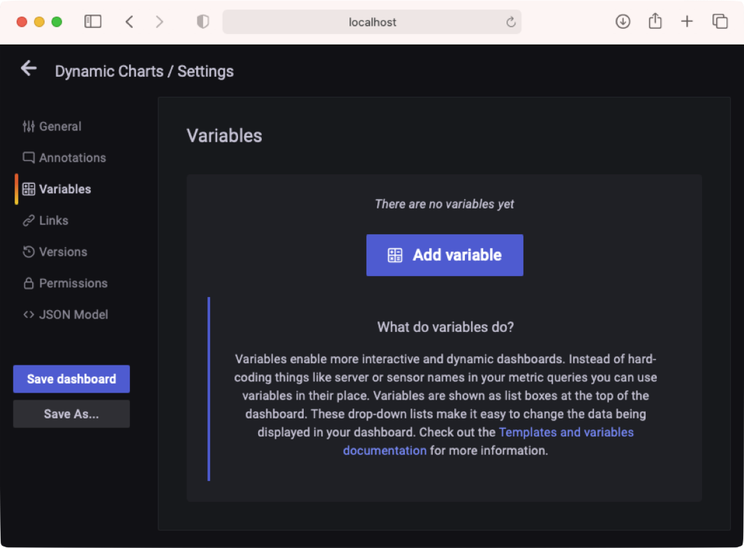
Click the Variables section on the left and then click Add variable (see Figure 30).

Figure 30: Add a variable to the current dashboard.

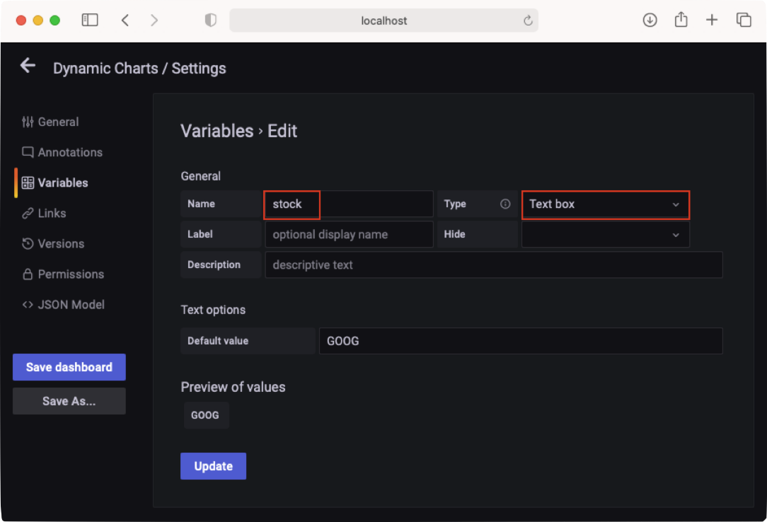
Enter the following information for the variable and then click Update (see Figure 31).

Figure 31: Configure the variable to be added to the dashboard.

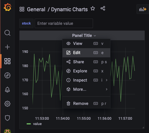
Back in the dashboard, select Edit for the panel (see Figure 32).

Figure 32: Editing the panel

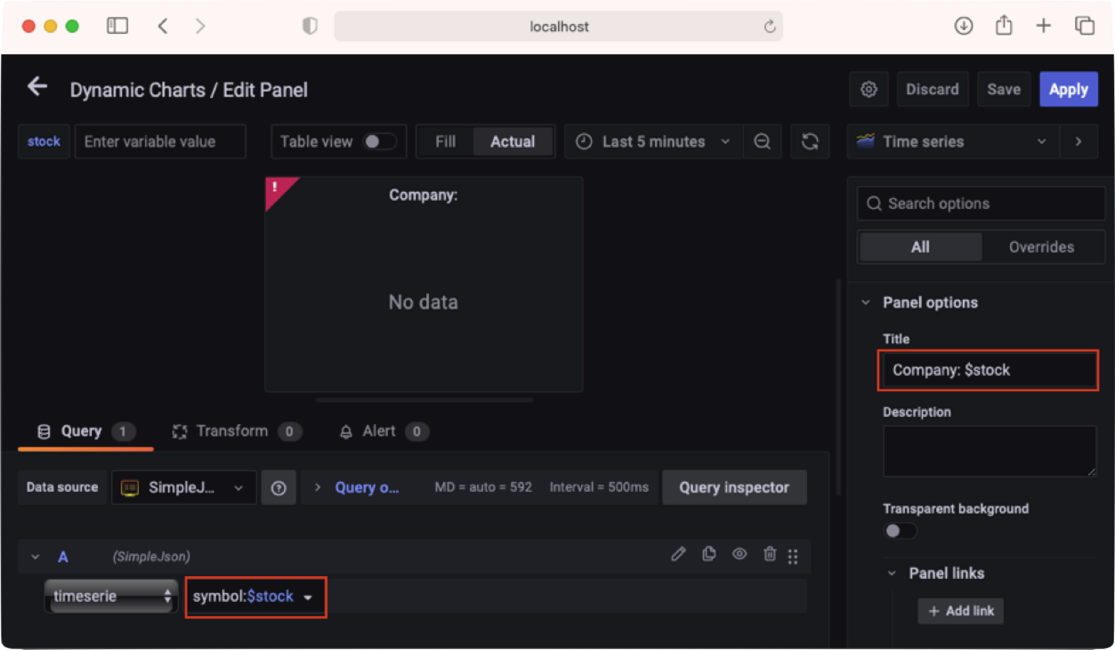
Set the title of the panel as Company: $stock and update the query to symbol:$stock (see Figure 33). Prefixing the variable name with the $ character allows you to retrieve the value of the variable and use it in your query and panel.

Figure 33: Using the newly added variable in the panel

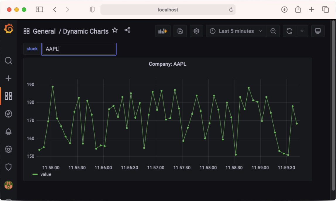
Click Apply. In the textbox next to the stock variable, enter AAPL. You should now see the chart for AAPL (see Figure 34).

Figure 34: Viewing the chart for AAPL

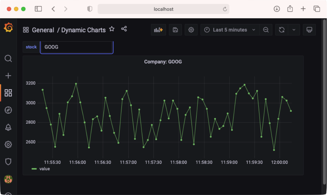
In the textbox next to the stock variable, enter GOOG. You should now see the chart for GOOG (see Figure 35).

Figure 35: Viewing the chart for GOOG

Auto-Updating the Chart

To automatically update the chart, select the drop-down list next to the Refresh button and select how often you want to refresh the chart (see Figure 36).

Figure 36: Select how often you want the chart to refresh.

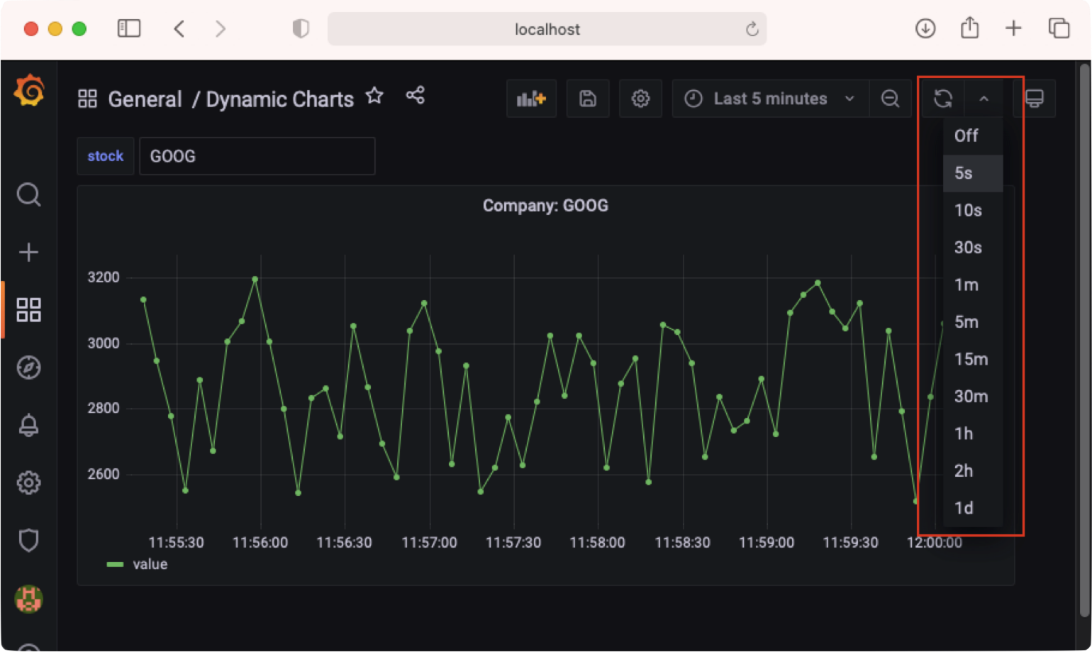
If you select 5s, the chart will now be updated every five seconds.

Displaying Real-Time Sensor Data Using MQTT

In Grafana 8.0, as part of the Grafana Live feature, it's now possible to perform real-time data updates using a new streaming API. This means that it's now possible for you to create charts that update in real-time and on-demand.

To make use of this feature, you can make use of the MQTT data source (https://github.com/svet-b/grafana-mqtt-datasource), a plug-in that allows Grafana users to visualize MQTT data in real-time. In this section, you'll learn how to use the MQTT data source to display sensor data in real-time.

In order to use the MQTT data source, you need to use Grafana 8.0, which makes it possible to perform real-time data updates using a new streaming API that's part of the Grafana Live feature.

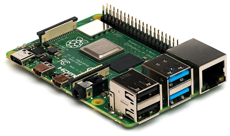
Using MQTT is ideal for projects such as those involving the Raspberry Pi (see Figure 37).

Figure 37: A Raspberry Pi

Installing the MQTT Data Source into Grafana

Although there is the MQTT data source built for Grafana, it doesn't come bundled with Grafana - you need to build and install it yourself. This is where the complexity comes in. In this section, I'll show you how to install the MQTT data source on Windows. You'll need a few tools/language:

• Node.js
• yarn
• Go
• Mage

Don't worry if you're not familiar with these tools and language. I'll show you how to install them in the following sections.

Install Node.js

Download and install Node.js from https://nodejs.org/en/download/. Once Node.js is installed on your system, type the following command in Command Prompt to install yarn:

npm install  - g yarn

Yarn is a package manager that doubles down as a project manager.

Install Go

Download and install Go from https://go.dev/dl/. Follow the instructions in the installer.

Go is a statically typed, compiled programming language designed at Google by Robert Griesemer, Rob Pike, and Ken Thompson.

Download Mage

Go to the source of Mage at https://github.com/magefile/mage. Click on the Code button and select Download ZIP (see Figure 38).

Figure 38: Download the source code for Mage.

Mage is a build tool like Make, but instead of writing bash code, Mage lets you write the logic in Go.

Once downloaded, extract the content of the zip file onto the Desktop. Next, find out the location of your GOPATH by typing this command in Command Prompt:

go env

You can locate the path for GOPATH from the output:

...
set GOOS=windows
set GOPATH=C:\Users\Wei-Meng Lee\go
set GOPRIVATE=
...

Type the following command to create a path call Go (if this path does not already exist on your computer; remember to use your own path):

cd c:\users\Wei Meng Lee\
mkdir Go

At the Command Prompt, change the directory to the mage-master folder:

cd C:\Users\Wei-Meng Lee\Desktop\mage-master

Type the following command:

go run bootstrap.go

You should see something like this:

Running target: Install
exec: go "env" "GOBIN"
exec: go "env" "GOPATH"
exec: git "rev-parse" " - short" "HEAD"
exec: git "describe" " - tags"
exec: go "build" "-o" "C:\\Users\\Wei-Meng
Lee\\go\\bin\\mage.exe" "-ldflags=-X\"github.com/magefile/
mage/mage.timestamp=2022-03-18T12:44:11+08:00\" -X
\"github.com/magefile/mage/mage.commitHash=\" -X
\"github.com/magefile/mage/mage.gitTag=dev\""
"github.com/magefile/mage"

Download the Source for the MQTT Data Source

The next step is to download the source code of the MQTT data source. Go to https://github.com/grafana/mqtt-datasource and download the ZIP file (see Figure 39).

Figure 39: Download the source code of the MQTT data source

Once the file is downloaded, extract the content of the zip file to the Desktop. Edit the file named package.go in the mqtt-datasource-main folder using a code editor. Replace "rm -rf dist && ..." with "del /F /Q dist && ..." (the command you replaced is to ensure that it works on Windows):

{
    "name": "grafana-mqtt-datasource",
    "version": "0.0.1-dev",
    "description": "MQTT Datasource Plugin",
    "scripts": { "build": "del /F /Q dist && grafana-
                  toolkit plugin:build && mage build:backend",
    ...

In the Command Prompt, cd to the mqtt-datasource-main folder:

cd C:\Users\Wei-Meng Lee\Desktop\mqtt-datasource-main

And type in the following commands:

yarn build
yarn install

Configuring the Plugin

Move the mqtt-datasource-main folder into the C:\Program Files\GrafanaLabs\grafana\data\plugins folder.

The C:\Program Files\GrafanaLabs\grafana\data\plugins folder is where Grafana stores the various plug-ins.

Next, load the defaults.ini file in the C:\Program Files\GrafanaLabs\grafana\conf folder and add in the following statement:

[plugins]
enable_alpha = false
app_tls_skip_verify_insecure = false
# Enter a comma-separated list of plugin identifiers
to identify plugins to load even if they are unsigned.
Plugins with modified signatures are never loaded.

allow_loading_unsigned_plugins = grafana-mqtt-datasource

# Enable or disable installing / uninstalling /
updating plugins directly from within Grafana.
plugin_admin_enabled = true

The above addition indicates to Grafana to allow unsigned plug-ins (which, in this case, is the MQTT data source). Restart Grafana in Windows Services. If you have performed the above steps in building the MQTT data source for Grafana, you should now be ready to use it.

Publishing Data to a MQTT Broker

Before you start to build a panel to display data using the MQTT data source, you need to write data to a MQTT broker so that you can subscribe to it. For this, I'll write a Python program to simulate some sensor data.

If you're not familiar with a MQTT broker, refer to my article on MQTT at: Using MQTT to Push Messages Across Devices.

Create a text file and name it publish.py. Populate it with the following statements:

# pip install paho-mqtt
import paho.mqtt.client as mqtt
import numpy as np
import time

MQTTBROKER = 'test.mosquitto.org'
PORT = 1883
TOPIC = "home/temp/room1/storeroom"

mqttc = mqtt.Client("python_pub")
mqttc.connect(MQTTBROKER, PORT)

while True:
    MESSAGE = str(np.random.uniform(20,30))
    mqttc.publish(TOPIC, MESSAGE)
    print("Published to " + MQTTBROKER + ': ' +
           TOPIC + ':' + MESSAGE)
    time.sleep(3)

The above Python program sends some data to the public MQTT broker every three seconds. To run the publish.py file, type the following commands in Command Prompt:

pip install paho-mqtt
python publish.py

Subscribe Using the MQTT Data Source

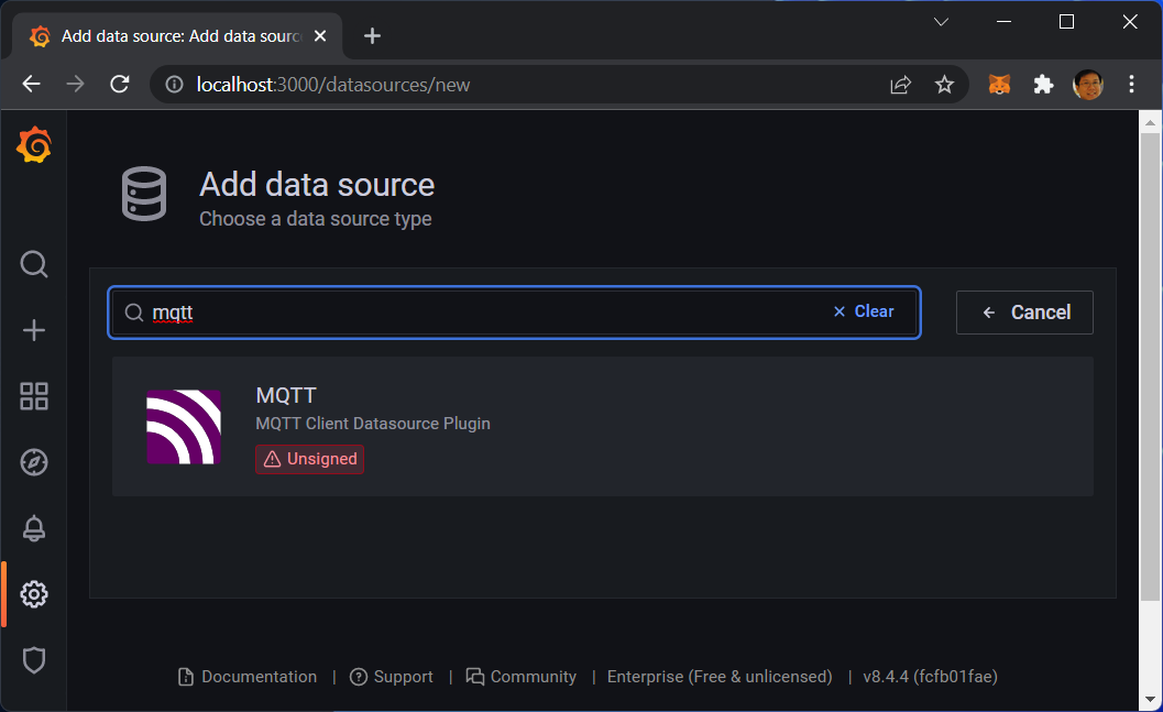
In Grafana, add a new data source by searching for mqtt (see Figure 40).

Figure 40: Add the MQTT data source to Grafana.

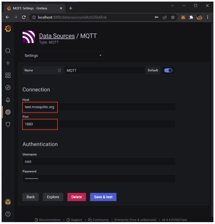
Configure the MQTT data source as follows (see also Figure 41):

• Host: test.mosquitto.org
• Port: 1883

You can leave the fields under the Authentication section empty. Click Save & test once you're done.

Figure 41: Configure the MQTT data source.

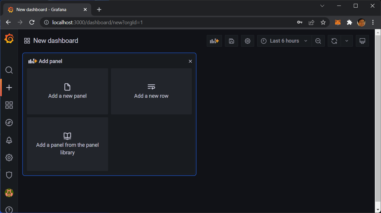
Next, create a new dashboard and add a new panel (see Figure 42):

Figure 42: Add a new panel to the dashboard.

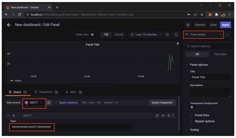
Configure the panel with the following (see also Figure 43):

• Visualization: Time Series
• Data source: MQTT
• Topic: home/temp/room1/storeroom

Click Apply when done.

Figure 43: Configuring the panel

You should now see the chart plotted and updated every three seconds (see Figure 44). If you can see the chart, this means that you're able to receive the data through the MQTT data source.

Figure 44: Display the data from MQTT as a line chart.

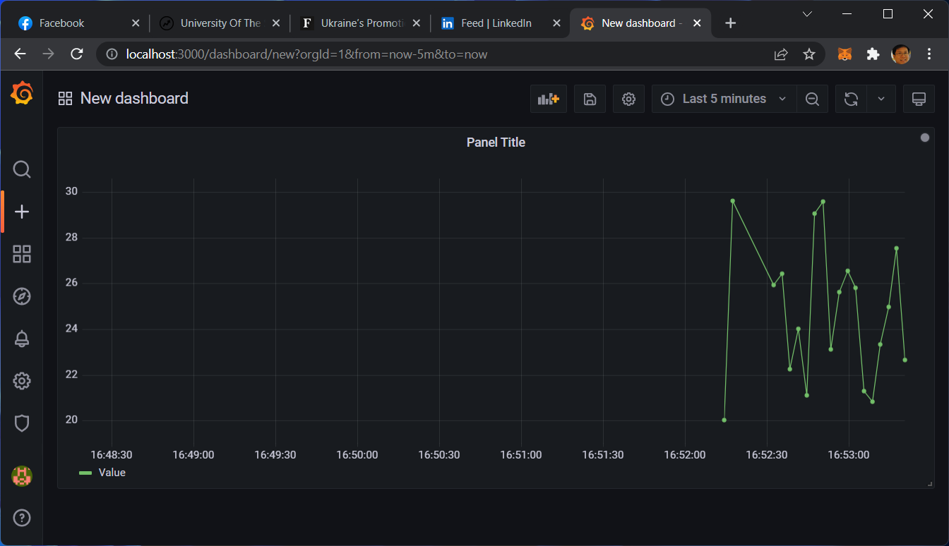
Hint: Switch the dashboard to view the Last 5 minutes to see a close-up of the chart.

Summary

In this article, you've seen how to use Grafana to build dashboards with a minimal amount of code needed. Instead of code, all you need is some basic SQL skills (of course, there will be cases where you need to write complex SQL queries to extract your data). In addition, I've walked you through two projects where you learned how to dynamically update your chart from a REST API, as well as fetch data from a MQTT data source. Have fun!